4 Manufacturing IoT: Maintenance and Supply Chains
More
Depth: Practitioner
Progress saves as you read. Mark sections complete as you go; your progress appears in the sidebar.
- Podcast audio coming soon
- Character narration audio coming soon
4.1 Turn Signals into Operating Decisions
Manufacturing IoT earns its place when machine measurements change maintenance, production, or supply decisions. A plant can collect useful production and packaging evidence while maintenance warnings and supply-chain signals still compete for attention. The team must connect each alert to an action, prove its return, and keep retail or logistics data from weakening factory reliability.
This is the second of two chapters; Manufacturing IoT: Plant and Packaging Evidence establishes the first part. Here, follow the plant’s maintenance problem through a line of 50 motors, then compare the same decision discipline with checkout and shelf monitoring. You will calculate predictive-maintenance value from stated evidence, connect retail and supply-chain sensing to decisions, and evaluate protocol, privacy, and deployment trade-offs.
The problem is choosing which evidence deserves intervention. A warning that never reaches a work order has little operational value, while an unreliable threshold can interrupt healthy equipment. Start with the maintenance trigger and its costs, then examine retail friction, product safety, and the architecture that connects evidence to action.
KEY CONCEPTS
- Condition evidence
Choose sensor trends that match the failure mode.
- Measured value
Separate avoided loss, gross benefit, and net ROI.
- Product safety
Carry product identity through to a recall decision.
- Workflows and boundaries
Link local control to maintenance and shared records.
4.2 Learning Objectives
By the end of this chapter, you will be able to:
- calculate predictive-maintenance value from stated evidence
- connect retail and supply-chain sensing to decisions
- evaluate protocol, privacy, and deployment trade-offs
4.3 Replace Calendar Guesses with Condition Evidence
The maintenance approaches differ in what starts the repair. Reactive maintenance fixes equipment after failure and has the highest cost profile in this comparison: unplanned downtime, emergency callouts, late parts, and damage to other components. Preventive maintenance replaces parts on a calendar or run-hour schedule. It buys planning at a medium cost, but can discard healthy parts and still miss early failures. Predictive maintenance (PdM) uses measured condition to schedule intervention as failure risk rises. Its intended lower-cost outcome is replacement when needed, fitted into downtime the plant already planned.
Figure 1 compares those triggers. Read it from left to right: the move toward predictive work depends on sensor trends, rather than the repair technique alone. The declining cost and downtime bands describe the comparison’s intended outcome, not a guaranteed result for every asset. The bottom strip identifies vibration, temperature, current, ultrasonic, and oil data streamed instead of sampled by hand.
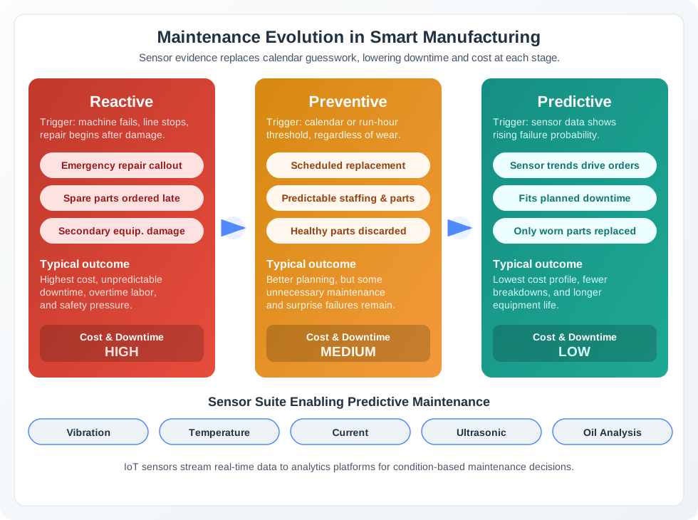
Choose sensors for the failure mode. Vibration reveals bearing wear, imbalance, and misalignment; temperature reveals motor overheating and bearing friction. Current measurements expose motor load and power-quality issues. Ultrasonic sensing can identify compressed-air leaks and electrical arcing, while oil analysis reveals contamination and wear particles. Together, these signals support condition evidence; their usefulness still depends on the machine’s operating context.
For functional predictive-maintenance programs, a US DOE guide reports survey-average estimates of 25–30% lower maintenance costs, 70–75% fewer breakdowns, 35–45% less downtime, and 20–25% higher production. Measure warning lead time and downtime reduction for each asset rather than treating those ranges as the plant’s forecast. Predictive Maintenance ML develops the vibration analysis and failure-prediction models behind this work.
4.4 Putting Numbers to It
Now put numbers against the 50-motor line. Each unplanned failure costs $15,000 in downtime and emergency repair. Reactive maintenance produces 8 failures per year; the predictive case assumes 2. Six avoided failures therefore save (8 − 2) × $15,000 = $90,000 annually. Vibration sensors cost $300 per motor once, and cloud analytics costs $150 per motor each year. First-year spending is 50 × ($300 + $150) = $22,500: $15,000 for sensors and $7,500 for analytics.
Net first-year return on investment, or ROI, subtracts spending before dividing by it: ($90,000 − $22,500) / $22,500 × 100% = 300%. Simple payback under these assumptions is about three months. After installation, modeled annual avoided-failure cost of $90,000 less $7,500 in analytics gives $82,500. These are illustrative results, dependent on the assumed failures and costs. The DOE program estimates provide context for measuring a functional program; they do not establish the failure reduction assumed for these motors. Connect the alert to manufacturing execution system (MES) work-order timing so the model corresponds to a maintenance decision.
4.5 Reduce Checkout Friction
After equipment reliability, consider the customer-facing side of the same problem: sensing pays when it changes a decision that reduces waiting, empty shelves, waste, or unsafe product use. The regional grocery chain has 45 stores and 450 self-checkout kiosks, averaging 10 kiosks per store. Customers complain about waits. Transactions average 3.2 minutes, abandonment is 18%, and the average self-checkout basket is $47.50.
The intervention combines weight sensors, barcode-scanner event loggers, and payment-terminal monitors to expose friction. Computer vision supports price look-up (PLU) codes for produce, while machine learning (ML) calibrates weight sensors to reduce false “unexpected item” alerts. Real-time queue monitoring directs attendants where help is needed. The practical target is fewer errors and easier item lookup, rather than faster transactions alone.
In the worked case, transaction time falls from 3.2 to 1.84 minutes, about a 42% reduction. Abandonment falls from 18% to 7%: an 11-percentage-point improvement, or about 61.1% relative. Keep those two ways of expressing change distinct when comparing interventions.
The annual recovered-revenue model input is $1,621,000, pending customer-volume and conversion assumptions. Dividing it by $112,500 in hardware investment gives 14.4x. That is recovered revenue divided by hardware spending, with operating costs excluded; it is not the net ROI calculated for the motors. The case’s strongest interventions target error prevention and item lookup automation, but the revenue claim still needs the missing volume and conversion evidence.
4.6 Find Stockouts While Restocking Still Helps
In this illustrative case, a specialty retailer has 120 locations, each carrying 8,500 active stock-keeping units (SKUs) across 1,200 shelf facings. The Baseline Out-of-Stock Rate is 8.3%, and Lost Sales per Hour per OOS is $4.20. Manual audits occur twice daily, taking 30 minutes each at $30 per hour; the Baseline Detection Rate is 60%.
The proposed response instruments high-velocity shelf locations for 400 SKUs per store with weight-based sensors. Each sensor costs $28, and Annual Cloud Cost per Sensor is $8. The model assumes 12 shopping hours per day and 365 days per year. Its Average OOS Duration input is 3.5 hours, but does not enter the calculation. Integration with the Warehouse Management System helps expose phantom inventory: stock recorded in the system that is unavailable on the shelf. Alert thresholds vary by product category. Instrumentation belongs where the hourly stockout loss justifies the sensor investment, rather than on every product indiscriminately.
With an IoT Detection Rate of 94%, a 34 percentage-point improvement from 60% to 94% detection, the illustrative model estimates $24,918,485.8 in annual recovered sales and $1,314,000 in labor savings from eliminated audits. The $1,728,000 year-one system cost includes sensors and annual cloud costs. Gross benefit is $26,232,485.8, about 15.2x the year-one cost; the $24,504,485.8 year-one net benefit divided by that cost is 14.2x. The model treats the detection improvement as recovered stockout time, an assumption that depends on timely restocking.
The standalone calculator uses these illustrative inputs and explores recovered sales, labor savings, sensor spending, and recurring cloud costs. Faster detection has value when it leads to restocking, just as a bearing alert has value when it reaches maintenance scheduling.
4.7 Mfg Retail IoT Check
The standalone checks retain the original interactive-check components for practice with the stated evidence.
4.8 Carry Product Identity Through to Safety Action
Retail sensing addresses availability; supply-chain visibility also has to address unsafe products. Figure 2 shows four responsibilities needed before a recall can stop a product at the point of use. Read from the bottom up, following the dependency between identity, communication, shared status, and local action.
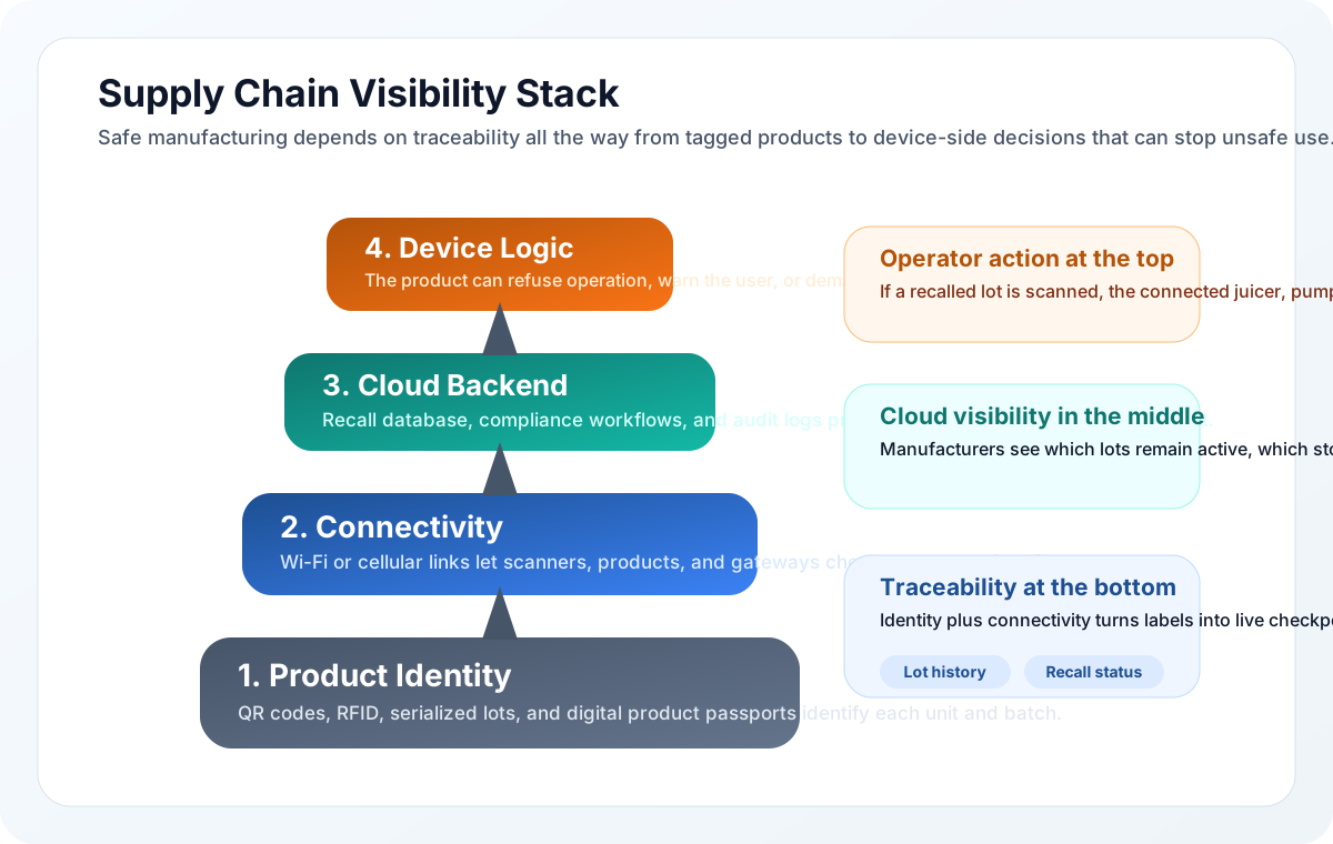
Product identity uses QR codes, serial codes, or radio-frequency identification (RFID) tags to track items or distinguish a batch from an entire product line. Connectivity through Wi-Fi or cellular service lets a scanner check that identity against recall information where the work happens. The cloud backend holds the recall database, compliance records, and audit trail, allowing safety alerts to propagate across sites. Device logic then changes behavior: it can refuse operation on a withdrawn lot instead of merely displaying a warning. A printed label becomes a live safety check only when the chain reaches that final decision.
Identity and condition are complementary. Time-temperature indicators show whether a package experienced a temperature excursion; freshness indicators and RFID/near-field communication (NFC) support condition or identity monitoring. Quantify prevented loss and waste reduction for the particular deployment. Cold-chain monitoring is the packaging connection, just as maintenance scheduling is the machine connection.
This connection extends beyond the plant. Healthcare IoT offers parallels in quality control and regulatory compliance. Smart Agriculture follows supply from farm to factory, while Smart Grid connects industrial energy management with optimization.
4.9 Put Each Decision Where Its Timing Can Be Met
The plant now needs an architecture that supports both immediate intervention and longer-term learning. Edge computing processes data near the machine. It supports local equipment control and safety responses, but requires local infrastructure and distributed algorithm deployment. Batch cloud analytics provides cross-facility patterns, more comprehensive analysis, and easier centralized updates; network delay makes it inappropriate for immediate control. Compare safety response requirements, connectivity reliability, algorithm complexity, and whether the objective is real-time control or strategic optimization.
The source’s sub-millisecond safety-response case and under-10-ms machine-stop target are requirements for particular control paths. They are different from the under-100-ms edge vibration-analysis latency below. Locating computation at the edge does not by itself establish a safe shutdown time. Edge Computing for IIoT develops this local-processing boundary.
4.10 Edge vs Cloud Vibration Analytics
The factory has 500 machines, each sampling vibration at 10 kHz. Fast Fourier Transform (FFT) analysis separates the signal into frequency components to detect bearing faults. Compare the stated options:
| Criterion | At the machine | Centralized cloud |
|---|---|---|
| Analysis latency | <100 ms; supports a prompt local response | 200–1000 ms network round-trip |
| Data sent onward | 10 Hz summaries; 99.9% reduction in sample rate | 10 kHz raw stream |
| Compute cost | $50–150 per machine | $5/month per machine |
| Algorithm updates | Update 500 devices | Update once centrally |
| Network outage | Local processing continues | Connectivity required |
| Cross-machine learning | Harder with siloed local data | Easier with centralized data |
| Initial investment | $25K–75K hardware | $2.5K setup |
| Stated five-year cost | $75K + $0 monthly = $75K | $2.5K + ($2.5K/month × 60) = $152.5K |
At 4 bytes per sample, 500 × 10,000 × 4 produces 20 MB/second before transport overhead. The 99.9% comparison describes sample rates, not a complete encoded-bandwidth budget.
Choose edge processing when a bearing-failure scenario allows only 30 seconds and requires detection within 100 ms, the floor has spotty connectivity, raw data volume is excessive, process control needs low latency, or a 5+ year deployment justifies upfront spending. Choose cloud when fleet-wide patterns matter, models change monthly, capital is limited, the factory has reliable wired/cellular connectivity, and hours or days of response time are acceptable. Monthly model changes still require coordinated deployment and rollback across 500 edge devices if processing stays local.
A hybrid design assigns FFT analysis, anomaly detection, and critical local shutdown decisions to the edge, sending 10 Hz summaries onward. Cloud processing combines machines’ summaries, trains ML models, and optimizes maintenance schedules, with a modeled prediction horizon of two weeks. The responsibilities address different parts of the maintenance workflow.
The example sensor samples at 10 kHz, or 10,000 points/second. The edge computer runs FFT analysis every 100 ms, with 1,024 frequency bins stated in the example. It detects a bearing signature at 180 Hz, with amplitude increasing 3x, then sends: “Machine 247, bearing outer race defect, 72 hours to failure.”
Cloud ML correlates the event with temperature, load, and maintenance history. The resulting recommendation is: “Schedule bearing replacement during next weekend shutdown.” The lead time is an example prediction to validate against the asset, not a guaranteed warning interval.
The cost-benefit assumptions assign $50K in avoided catastrophic machine damage to local detection. Cloud scheduling is assumed to reduce unplanned downtime costs by 40%, or $120K/year, from an implied $300K/year baseline.
The source also gives GE Predix as an industrial hybrid example: real-time vibration analysis on turbine controllers, with cloud fleet analytics across 10,000+ turbines globally. It attributes blade-crack predictions two weeks before failure and $100M annually in avoided unplanned downtime to that example. These source claims have no supporting citation here; they require verification before use in a business case.
4.11 Industrial Protocol Tradeoff
Protocol selection must support those responsibilities. A vendor’s proprietary protocol may offer optimized performance, integrated support, and equipment communication, while increasing lock-in and integration complexity. OPC UA offers vendor-neutral interoperability and long-term flexibility, with possible performance compromises and varying implementation quality. Assess the installed base, vendor relationships, the actual multi-vendor environment, and the strategic value of data portability. Industrial Networking and Protocols connects Modbus, OPC UA, and industrial Ethernet to these choices.
4.12 Deploy Evidence Without Creating New Operational Risks
Architecture succeeds when evidence reaches existing work. A new condition-monitoring dashboard can create a data silo if it bypasses enterprise resource planning (ERP), MES, and quality systems. Vendors often optimize for quick platform deployment, while information technology (IT) and operational technology (OT) teams have competing priorities. Require an API-first architecture, with defined application programming interfaces for integration, and governance spanning both domains. Estimate the actual ERP, MES, and quality-system interface costs before approving the budget. Test that alerts reach maintenance, production, and quality workflows.
Start with historical downtime and the highest-cost failure modes, then instrument critical machines. Thresholds need 4–8 weeks of observe-only baseline data before alerts are activated. Normal operating variation otherwise creates false alarms until operators learn to ignore them. Two nominally identical motors can have different vibration signatures because of installation, wear history, and load profiles. Calibrate each asset individually and store its baseline in the maintenance database. Train anomaly detection against that context, then integrate alerts with scheduling and automated work orders.
Privacy also needs a boundary before rollout. Incremental worker-location, productivity, or biometric tracking without transparent policies can provoke employee pushback, union grievances, and legal challenges. Communicate policies before deployment, aggregate location data instead of retaining individual trails, set retention limits, and involve employee representatives in system design. A fast proprietary machine link does not resolve either data portability or permission to track workers.
Finally, IT practices cannot simply be transferred to OT. Frequent patches or antivirus scans can disrupt real-time control systems designed around reliability. Use the source’s demilitarized-zone (DMZ) architecture and data-diode boundary between OT and IT, following the IEC 62443 zone and conduit security model. The boundary keeps control ownership visible as data moves toward analytics. Manufacturing draws together industrial sensors (Module 2), Modbus/OPC UA (Module 3), edge processing for programmable logic controller (PLC) integration (Module 5), and secure OT networks (Module 7).
Summary
Predictive maintenance connects condition evidence to work before a breakdown. The DOE guide supplies program-level comparisons, while the motor example yields 300% net first-year ROI under its assumptions; the retail examples mainly report gross benefit or recovered revenue relative to investment, and the smart-shelf case states both its 15.2x gross ratio and its 14.2x net figure. Preserve those distinctions when comparing value, and validate reductions in downtime, waste, or lost sales for the deployment.
Supply visibility connects identity, connectivity, cloud records, and device logic so a recall can change behavior. Edge processing supports local decisions; cloud analytics supports fleet learning and scheduling. Both depend on per-asset baselines, protocol portability, privacy rules, OT boundaries, and budgeted ERP/MES and quality-system integration.
Connect each measurement to a production or maintenance decision, with evidence that the action happened. Prioritize reliability, OT safety, and plant workflows when adding analytics.
Continue with Industrial Networking and Protocols to examine the communication choices behind these operating decisions.