7 IoT Financial Metrics: Forecasting and TCO
More
Depth: Practitioner
Progress saves as you read. Mark sections complete as you go; your progress appears in the sidebar.
- Podcast audio coming soon
- Character narration audio coming soon
7.1 Forecast the Whole Business
The unit-economics calculation passes on today’s inputs, but the team still has to fund growth. Adoption, churn, support, cloud, and replacement costs can move after the decision. This chapter builds revenue and cost projections, compares lifecycle ownership costs, and tests whether a financial decision survives changes in its assumptions.
Return to the smart thermostat company: a healthy customer ratio can encourage acquisition long before subscription payments recover the cash spent upfront. The same problem appears when a platform quote omits the integration and operating work needed to serve those customers. The team needs a forecast that exposes both gaps.
This is part 2 of 2. Review IoT Financial Metrics: Unit Economics for the foundation. In the linked figure in Part 1, the improvement levers meet at business viability. Here, keep their measures tied to the same cohort, a group of customers tracked together: lifetime value (LTV), customer acquisition cost (CAC), average revenue per user or account (ARPU), and churn must describe that same group.
The problem is turning a promising ratio into an affordable operating plan. First project retained customers and revenue; then account for platform and integration costs; finally test cohort value and cash timing before choosing how fast to grow.
KEY CONCEPTS
- Growth assumptions
New customers and churn determine the paying base.
- Lifecycle cost
The first invoice leaves operating and integration costs open.
- Cohort value
Retention and margin determine customer contribution.
- Cash timing
Acquisition is paid before subscription margin repays it.
7.2 Learning Objectives
By the end of this chapter, you will be able to:
- build an IoT revenue and cost projection
- compare alternatives with lifecycle total cost
- test financial decisions with sensitivity evidence
7.3 Project Customers Before Revenue
A growth forecast starts with the active customer base. Each month, remove customers who churn, add newly acquired customers, and multiply the resulting base by monthly ARPU. Apply the gross margin to estimate contribution before acquisition spending and other overhead; calling this bottom-line profit would hide the remaining costs.
The revenue calculator starts with 10 customers, adds 5 each month, and assumes $500 monthly ARPU, 3% monthly churn, and 75% gross margin over 12 months. Its rule is next customers = current customers × 0.97 + 5. The first two modeled customer counts are 14.7 and 19.259. Fractional counts represent an expected base; rounding the displayed count should not change the revenue calculation.
Under these fixed assumptions, additions initially exceed churn and monthly contribution rises. Acquisition and churn would balance near 167 customers, where 3% of the base is about 5. That is a model boundary, not evidence that acquisition or retention will remain fixed. Compare final monthly revenue and contribution with their cumulative totals before treating growth as cash available to spend.
The forecast checks growth under one set of assumptions. Next ask whether its cost structure still works when device count, message volume, storage, support, and integrations arrive.
7.4 Count the Lifecycle Cost
Total cost of ownership (TCO) covers the costs of buying and operating the deployment across its lifecycle. Hardware, connectivity, cloud operations, maintenance, support, and integration accumulate across years, well beyond the initial quote.
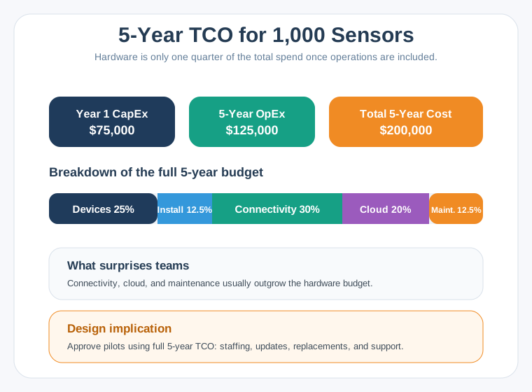
The 1,000-sensor example in Figure 1 separates $75,000 of year-one capital spending from $125,000 of five-year operating spending: $200,000 altogether. The purchase commitment covers barely more than a third of that total. Connectivity takes 30%, devices 25%, and cloud 20%; installation and maintenance share the remainder. Recurring categories outgrow hardware, so a forecast based on device price can run short in year two.
For a separate 10,000-device deployment, the following are worked-example pricing assumptions, not current vendor quotations. Keep the units explicit: per-device charges, message volume, storage, dashboards, and support contribute differently.
| Cost Category | Vendor A (AWS IoT) | Vendor B (Azure IoT) | Vendor C (Specialist Platform) |
|---|---|---|---|
| Platform Base | $0 (pay-per-use) | $0 (pay-per-use) | $50,000/year |
| Device Connections | $0.08/device/month = $9,600/yr | $0.10/device/month = $12,000/yr | Included |
| Message Ingestion | $1.00/M messages | $1.50/M messages | Included up to 100M |
| Data Storage | $0.023/GB (S3) | $0.018/GB (Blob) | $0.05/GB |
| Analytics/Rules | $0.15/M rule evaluations | $0.20/M rule executions | Included |
| Dashboards | Additional service ($500/mo) | Power BI ($10/user/mo) | Included (5 users) |
| Support | Business: $15K/yr | Professional: $12K/yr | Premium: $20K/yr |
At 288 messages per device per day, a five-minute reporting interval, the monthly volume is 10,000 × 288 × 30 = 86.4M messages. With the table’s assumptions, ingestion alone costs $86.40/month for AWS IoT Core and $129.60/month for Azure IoT Hub. The specialist’s message charge is $0 within its included allowance, with the platform fee still payable. None of these ingestion figures is the whole monthly bill.
The five-year comparison adds a lifecycle view:
| Year | AWS IoT | Azure IoT | Specialist Platform |
|---|---|---|---|
| Year 1 | $185,000 | $210,000 | $145,000 |
| Year 2 | $165,000 | $188,000 | $120,000 |
| Year 3 | $175,000 | $195,000 | $130,000 |
| Year 4 | $190,000 | $205,000 | $140,000 |
| Year 5 | $210,000 | $220,000 | $150,000 |
| 5-Year Total | $925,000 | $1,018,000 | $685,000 |
| Monthly per Device | $1.54 | $1.70 | $1.14 |
These scenario totals are $925,000, $1,018,000, and $685,000, or $1.54, $1.70, and $1.14 per device per month across five years. They are broader budget assumptions, not totals derivable from the ingestion calculation alone. Specialist platforms trade some flexibility for domain capability and potentially lower TCO; hyperscalers offer more services, but separate service charges accumulate.
7.5 Budget Integration Before Selecting a Platform
The cost comparison is incomplete until the team budgets implementation. At a blended $150/hour, Year 1 integration has the following range. Training and ongoing maintenance also belong in the deployment estimate.
| Integration Component | Time Estimate | Cost ($150/hr blended rate) |
|---|---|---|
| Device provisioning workflow | 80-120 hours | $12,000-$18,000 |
| Data model design and implementation | 60-100 hours | $9,000-$15,000 |
| Dashboard/visualization development | 120-200 hours | $18,000-$30,000 |
| Alert/notification system | 40-80 hours | $6,000-$12,000 |
| ERP/CRM integration | 160-300 hours | $24,000-$45,000 |
| Security implementation | 80-160 hours | $12,000-$24,000 |
| Testing and validation | 80-120 hours | $12,000-$18,000 |
| Documentation and training | 40-60 hours | $6,000-$9,000 |
| Total Integration | 660-1,140 hrs | $99,000-$171,000 |
Figure 2 starts with the binding constraint: scale, enterprise integration, analytics, control, or a quick prototype. Its product examples include Amazon Web Services (AWS) IoT Core, Azure IoT Hub, Google Cloud, custom MQTT, and ThingsBoard. The implementation range of 660–1,140 hours and $99,000–$171,000 remains relevant whichever route is chosen.
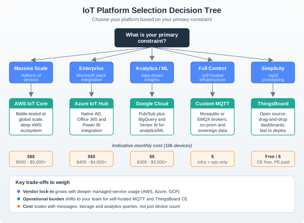
Choose a hyperscaler (AWS/Azure/GCP) when broad ecosystem integration matters: AI/ML, data lakes, and enterprise applications require identity, data, and service connections the team can support. Cloud expertise, unpredictable or highly variable workloads, and a long-term strategic cloud commitment strengthen that case.
Choose a specialist when domain expertise in industry, healthcare, or agriculture matters, predictable load supports fixed pricing, and time-to-value takes priority over flexibility. Limited internal IoT engineering capacity also favors this route. Build your own when platform control is the competitive advantage, commercial platforms miss unique requirements, scale justifies the engineering investment (100K+ devices), and the organization can sustain a 5+ year commitment.
Platform choice also distributes value among device manufacturers, connectivity providers, platform operators, and developers. Their incentives differ: hardware volume, stable traffic, transaction fees, and affordable application access must fit together. Revenue sharing, standardized APIs, integration protocols, and clear governance reduce that friction; uniform fees can ignore different cost structures. The ecosystem exercise uses 15–30% platform fees and a 70–85% developer share as illustrative splits.
7.6 Stress-Test Subscription Cohorts
The platform decision is only one failure mode. Churn, subsidies, and pricing can change customer value even after the operating cost model is complete.
Peloton reported Connected Fitness churn rates of 0.65% in Q1 FY21 and 1.41% in Q4 FY22. Those reported rates are inputs from different quarters; all ARPU, CAC, hardware, and cohort values below are hypothetical model assumptions.
Modeled peak cohort (using Peloton Q1 FY21 reported churn as one input):
| Metric | Value | Assessment |
|---|---|---|
| Monthly ARPU | $99 (assumption) | Hypothetical subscription ARPU; hardware cash flows excluded |
| Monthly churn | 0.65% (Peloton Q1 FY21 reported Connected Fitness churn; used here as a model input) | Implies about 12.8 years under a constant-churn model |
| LTV | $99/month / 0.0065 = $15,231 | At assumed 60% margin, contribution LTV is about $9,139 |
| CAC | ~$1,600 (assumption) | Modeled LTV:CAC ratio = 5.7:1 |
| Payback period | $1,600 / ($99 x 0.60) = 27 months | Scenario payback, excluding hardware cash flows |
At these assumed metrics, the business model would look attractive. Peloton invested in manufacturing capacity and content studios, and acquired Precor for $420 million in cash.
Modeled later cohort (using Peloton Q4 FY22 reported churn as one input):
| Metric | Value | Change |
|---|---|---|
| Monthly ARPU | $44 (assumption) | -56% from the modeled $99 subscription ARPU |
| Monthly churn | 1.41% (Peloton Q4 FY22 reported Connected Fitness churn; used here as a model input) | +0.76 percentage points; about 117% relative to 0.65% |
| LTV | $44/month / 0.0141 = $3,121 | -79% from the modeled $15,231 revenue LTV |
| CAC | ~$1,800 (assumption) | +12.5% from the modeled $1,600 |
| LTV:CAC ratio | $3,121 x 0.60 / $1,800 = 1.04:1 | Below a modeled 3:1 planning target |
| Payback period | $1,800 / ($44 x 0.60) = 68 months | About 5.7 years in this simplified model |
What the hypothetical cohorts illustrate:
-
Hardware subsidy trap: In this hypothetical cohort, any upfront hardware subsidy must be recovered from future subscription contribution; calculate the actual subsidy and churn sensitivity before scaling.
-
Churn sensitivity: Using Peloton-reported churn rates from Q1 FY21 (0.65%) and Q4 FY22 (1.41%) as inputs, this hypothetical cohort, with lower assumed ARPU, reduces modeled revenue LTV from $15,231 to $3,121. These are not Peloton-reported customer values.
-
Hardware does not guarantee retention: Even $2,000 of connected hardware in a customer’s home does not establish permanent subscription lock-in. A customer can stop using the bike and cancel the service. The hypothetical cohort illustrates that risk; it does not establish what Peloton assumed about customer behavior.
Lesson for IoT businesses: Test whether subscription contribution margin repays any hardware subsidy before customers leave. Stress-test at 2x and 3x the observed churn rate. Treat 3:1 LTV:CAC as a planning screen, then check payback and cash needs for your margins.
7.7 Put a Horizon on Smart-Building Value
Now apply retention to the commercial-building heating, ventilation and air conditioning (HVAC) control platform. Monthly ARPU is $450: a $350 platform fee and $100 average add-on modules. The SaaS platform assumes low cost of goods sold and 72% gross margin, 1.8% monthly churn (98.2% retention), and an $8,000 setup fee collected once in year one. The question is whether five years of contribution justify acquisition spending.
Bill month one at full retention. Monthly contribution is $450 × 0.72 = $324.00 initially, $318.17 in month two, and $312.44 in month three. By month 60, it is $324 × 0.982^59 = $110.95. Summing retained contribution over months 1–60 gives $11,947.12; applying the assumed 72% margin to setup adds $5,760. Total five-year contribution LTV is therefore $17,707.12.
For monthly retention r and a horizon of H months, recurring contribution is ARPU × margin × Σ(r^i), with i from 0 to H−1. Equivalently, for r ≠ 1 it is ARPU × margin × (1−r^H)/(1−r). Month one uses exponent zero because it is fully retained.
For this building, an Excel expression is =450*0.72*SUMPRODUCT(0.982^(ROW(A1:A60)-1)). Using exponents 1–60 would apply churn before the first billed month. Keep this finite-horizon estimate separate from an uncapped 1/churn average lifetime.
With $17,707.12 LTV, a 3:1 screen permits about $5,902 CAC; a 5:1 target permits about $3,541. Current CAC of $6,200 produces approximately 2.86:1, below the 3:1 planning screen. The forecast needs improvement before it can support the earlier growth argument.
At hypothetical 3% churn, recurring contribution over the same 60 months falls to $9,063.29. Keeping churn at 1.8% adds about $2,884, with setup unchanged. That is the modeled value available to weigh against customer-success spending; it does not mean any retention intervention pays for itself.
7.8 Match the Revenue Model to the Constraint
The cohort calculations help evaluate the choices in IoT Business Model Fundamentals. Compare revenue potential, risk, and resource requirements together. The ranges below describe the chapter’s illustrative model comparison; each proposal still needs measured cohort costs and retention.
| Criterion | Hardware Sales | Platform-as-a-Service (PaaS) | Data Monetization | Hybrid (Hardware + Subscription) |
|---|---|---|---|---|
| Upfront revenue | High ($500-5K per unit) | Low ($0-500 setup) | Very low ($0) | Medium ($200-2K hardware) |
| Recurring revenue | None | High ($20-500/mo) | Medium ($5-50/mo) | High ($10-200/mo) |
| LTV:CAC potential | 1:1 to 2:1 (low) | 5:1 to 15:1 (excellent) | 3:1 to 8:1 (good) | 4:1 to 10:1 (very good) |
| Churn impact | N/A (one-time sale) | Model from subscriber cohorts | Model from buyer cohorts | Model from hardware and subscription cohorts |
| Cash flow | Depends on sale and production timing | Depends on CAC and payback | Depends on buyer ramp | Depends on hardware and recurring margin |
| Gross margin | Calculate from device costs | Calculate from service costs | Calculate from data-product costs | Calculate from blended costs |
| Customer lock-in | Low (purchase complete) | Medium (switching cost) | High (data network effects) | Very high (hardware + data) |
| Scalability | Limited (manufacturing) | Excellent (SaaS) | Excellent (marginal cost ~$0) | Good (hardware bottleneck) |
| Best for | Low-tech buyers, one-time need | Enterprise customers, predictable workloads | API consumers, data-driven orgs | Consumer IoT, SMB markets |
Ask whether customers can be retained for 3+ years: that supports PaaS or hybrid, while a one-time need favors hardware sales. Ongoing service value points toward PaaS; one-time capability points toward hardware. Defensible data valuable to third parties supports data monetization; otherwise focus on platform or hardware.
Capital and competitive advantage narrow the choice further. High available capital can support long PaaS payback; limited capital favors earlier hardware or hybrid cash receipts. Software/IP points toward PaaS, manufacturing toward hardware, and network effects toward data.
In this example, a smart agriculture startup chooses a hybrid model: it sells soil sensors for $150 at an assumed 20% hardware gross margin, then charges $25/month for irrigation management. The 18-month payback and four-year customer lifetime are scenario assumptions.
Validate the table’s lock-in and scalability expectations against actual cohorts. ARPU and churn supply evidence about product-market fit. Case Studies applies financial analysis to Philips, Amazon, and John Deere.
7.9 Check the Cash Gap Before Scaling
Return to the smart thermostat company. It celebrates a 5:1 LTV:CAC ratio ($1,200 LTV / $240 CAC), increases acquisition from 500 toward 5,000 customers per month, then runs out of cash six months later and needs emergency funding at a down round. The ratio describes eventual customer value; it does not fund today’s acquisition.
Payback period is the time required for customer contribution to recover acquisition cost. Here, CAC / (ARPU × gross margin) = \$240 / (\$15 × 0.70) = 22.9 months. Spend $240 at month zero on sales, marketing, and onboarding; collect $10.50 monthly contribution in months 1–22; simple payback arrives in month 23, assuming the customer remains active.
The first three acquisition cohorts expose the gap. Following the illustration’s convention, contribution starts in the month after acquisition and these rows omit churn:
| Month | New customers | CAC spend | Monthly contribution from earlier cohorts | Net cash flow |
|---|---|---|---|---|
| 1 | 500 | −$120,000 | $0 | −$120,000 |
| 2 | 1,000 | −$240,000 | $5,250 (500 × $10.50) | −$234,750 |
| 3 | 2,000 | −$480,000 | $15,750 (1,500 × $10.50) | −$464,250 |
At 5,000 acquisitions per month, CAC spending alone reaches $1.2M/month. Month 6, 12, and 18 balances require the missing acquisition schedule and retained counts; a cumulative count of customer-months cannot be treated as active customers paying in one month. Sum monthly net cash flows to find peak funding need before claiming a cumulative burn or a first positive month.
As a rough spending envelope, $1.2M/month × 22 months is $26.4M. That multiplication is not the required working capital: it omits contribution collected during the ramp and does not specify churn or the acquisition schedule. Raise capital against the cohort cash forecast before scaling. Reducing CAC from $240 to $180 cuts simple payback from 22.9 to 17.1 months and saves $300,000 of upfront acquisition spending each month at 5,000 acquisitions.
Use the chapter’s general payback screen of less than 18 months alongside its tighter planning targets: less than 12 months for VC-funded growth and less than 6 months for bootstrapped growth. These are screens to test against the business’s funding and margins. Even a 5:1 ratio can create a cash crisis when contribution arrives over 18–24 months.
Calculate LTV and payback from contribution after cost-to-serve. Subscription price alone hides device subsidy, connectivity, storage, support, warranty, payment fees, and field operations. Video retention, cellular traffic, support calls, or truck rolls can consume an apparently attractive margin. Compliance, training, replacement, and operational savings also belong in the lifecycle business case.
Portfolio averages can hide failing cohorts: self-serve SMB customers, enterprise pilots, reseller-led deals, and subsidized bundles can have different CAC, activation, churn, support load, and expansion paths. Review those differences before changing pricing, channel spending, or onboarding. At fixed monthly contribution, the uncapped constant-churn estimate gives average lifetime 1 / monthly churn: 2% versus 5% is a 3-percentage-point gap and a 2.5× lifetime difference. Retention changes the number of contributing months; ARPU changes their revenue rate. Compare both changes on the same horizon rather than assuming retention always wins.
Summary
A financial forecast joins retained customers, revenue, operating cost, integration, and acquisition spending. Compare alternatives over the same lifecycle, and keep reported company inputs distinct from hypothetical assumptions. TCO includes the work needed to run the deployment, not just the platform invoice.
Use 3:1 LTV:CAC as a planning screen and 5:1+ as evidence of stronger modeled unit economics, then check payback and available cash. A ratio below 3:1 calls for review; even one above 5:1 cannot authorize aggressive growth without funding evidence. The smart-building sum and thermostat cash gap show why the arithmetic and timing must reconcile before the team scales.
Include hardware, connectivity, cloud, support, churn, replacement, and operational savings across the lifecycle. Pair customer value with payback and cohort cash flow before committing to growth.
Continue to Go-to-Market Strategy to connect CAC, acquisition channels, and pricing to a B2B launch plan.