10  Lab: Routing Algorithms by Hand

Keywords

routing algorithms lab, longest prefix match, Dijkstra, Bellman-Ford, distance vector, link state, split horizon, RPL objective function

10.1 Start With a Candidate Path

A routing algorithm is easier to understand when you ask it to choose between candidate paths. One path may have fewer hops, another may have better link quality, and another may avoid a device that should not carry relay traffic.

The useful lesson is not the formula alone. The useful lesson is how the algorithm turns evidence into a next-hop decision, and how a reviewer can tell whether that decision still fits the network after conditions change.

10.2 In 60 Seconds

Routing algorithms are best learned as traceable decisions, not as long copied programs. This lab asks you to trace three algorithm families: longest-prefix match for forwarding lookup, Dijkstra-style shortest-path computation for link-state routing, and Bellman-Ford-style distance-vector rounds for neighbor-based routing. The output should be a decision record showing candidates, selected route, path weight, convergence round, loop-control behavior, and any limits of the model.

10.3 Learning Objectives

By the end of this chapter, you will be able to:

• Trace longest-prefix match before comparing ordinary route metrics.
• Run a small Dijkstra-style shortest-path lab and explain the selected next hop.
• Run distance-vector update rounds and identify when the table has converged.
• Explain split horizon and poison reverse as loop-reduction behavior.
• Compare link-state and distance-vector methods without overstating either one.
• Relate algorithm choices to constrained IoT routing and RPL objective functions.

Quick Check: Algorithm Trace Boundaries

10.4 Lab Scope and Trace Rules

You may use Python, a spreadsheet, a graph worksheet, or a simulator. Keep the lab record small enough to inspect. Do not paste long source listings into the report. Instead, record inputs, intermediate decisions, and final outputs.

Each algorithm lab should include:

• The topology or route table being tested.
• The decision rule being applied.
• The intermediate candidates that were rejected.
• The final selected route, next hop, or path.
• The reason the decision is valid.
• A limitation note stating what the model does not prove.

Overview: Algorithms Are Decision Records

A routing algorithm lab is useful when it makes each choice inspectable. Longest-prefix match should show every candidate prefix before the winner. A Dijkstra trace should show the settled set, frontier entries, improved tentative paths, and next-hop derivation. A distance-vector lab should show neighbor reports, update rounds, stale entries, and loop-control behavior.

Three algorithm labs need three visible records: prefix filtering for lookup, frontier updates for link-state reasoning, and update rounds plus withdrawal evidence for distance-vector convergence.

The common thread is not the algorithm name. The common thread is the record that explains why one route, parent, or next hop was accepted while other candidates were rejected. Without that record, a final path can look correct while hiding a stale route, a missing return path, or a metric choice that would fail under a small topology change.

Read each record from the question to the decision. A lookup record starts with the destination address, not with the route that looks attractive. A Dijkstra record starts with the source and the current frontier, not with the final shortest-path tree. A distance-vector record starts with what each neighbor advertised in that round, not with a table copied after convergence. This ordering matters because it makes a wrong turn visible: a metric compared too early, a tentative path accepted too soon, or a stale neighbor report kept after a failure.

The lab is also teaching scope. These algorithms can explain a selected next hop or computed path, but they do not by themselves prove packet delivery, return reachability, security policy, radio reliability, or RPL parent stability. Put those claims in separate rows when they are tested. That habit keeps a small classroom trace honest and prepares the same record style for real constrained-network review.

• Lookup proof: list matching prefixes before route source or metric comparisons.
• Graph proof: show settled nodes, frontier updates, improved paths, and next-hop extraction.
• Convergence proof: record update rounds, withdrawals, loop-control rules, and the stop condition.

Practitioner: Build The Algorithm Lab Record

Use one table for the lab result: input state, decision rule, rejected candidates, selected route, packet or control-plane implication, and limitation. That structure keeps the report short while still proving the reasoning. It also makes errors easy to find, because a missing candidate or skipped round becomes visible.

Keep the table at the same grain as the decision. For longest-prefix match, one row can be one destination lookup with all matching prefixes listed in order. For Dijkstra, one row can be one iteration: node settled, frontier before the step, changed tentative distances, and predecessor updates. For distance-vector, one row can be one exchange round: neighbor advertisement, local calculation, accepted change, rejected stale route, and loop-control rule. Mixing those grains in one row makes the record harder to audit because a reader cannot tell which evidence caused which decision.

For constrained IoT routing, add one extra column: cost of maintaining the record. Link-state knowledge can require more topology state. Distance-vector knowledge depends on neighbor reports and timers. RPL parent choice depends on Rank, Objective Function behavior, Trickle timing, DAO state, and observed forwarding. Those maintenance costs are part of the design decision.

When a lab names RPL variants, keep the record concrete. CORPL keeps the RPL DODAG idea but uses a forwarding set rather than one fixed parent for some traffic, while CARP is a channel-aware distributed routing approach for constrained wireless nodes. Those labels are comparison cues; the accepted route still needs metric, parent or forwarding-set, link-quality, and packet evidence.

Use practical labels rather than mathematical shorthand alone. "R4 improved from 5 through R3 to 4" is easier to inspect than a copied formula with no route name. "R1 suppresses the route learned from R2 when advertising back to R2" is clearer than only writing "split horizon." When the lab uses a spreadsheet or script, keep the inputs and changed rows in the report and link the script separately. A good practitioner record lets someone reproduce the decision without reading hundreds of lines of code.

The limitation column should be specific. Write "does not prove return path after withdrawal" or "does not model triggered-update timer" instead of "simulation only." In an IoT design review, that limitation becomes the next test: packet trace, parent-stability observation, DAO evidence, or border-router check. The algorithm table is therefore not the whole release record; it is the part that proves the route-selection reasoning.

• Before the run: name the topology, destination scope, route source, and metric or objective rule.
• During the run: keep intermediate candidates, changed weights, and invalidated paths.
• After the run: state what the trace proves and which field behavior still needs packet evidence.

Under The Hood: Convergence Is Shared State

Convergence means routers have reached a stable enough shared view for the tested condition. It is not guaranteed by one final table. A route can be locally selected while a neighbor still advertises stale information, a return path is absent, or a loop-control rule has not removed a bad path yet.

Different algorithms make different promises about that shared state. In a link-state model, each router is assumed to have a current view of the topology before it runs shortest-path-first. The interesting evidence is how that topology view was learned, whether stale link-state information was rejected, and when the SPF result was installed into forwarding. In a distance-vector model, the router does not need the whole topology, but it depends on neighbor reports. The interesting evidence is the update round, the metric calculation through each neighbor, and the rule that prevents a bad route from being advertised back as if it were useful.

This is why the lab separates algorithmic rules from protocol behavior. Dijkstra describes a shortest-path calculation over known topology. Bellman-Ford describes updates from neighbor distance reports. Real routing protocols add timers, triggered updates, hold-down behavior, sequence numbers, policies, authentication, and implementation limits. RPL adds DODAG structure and low-power control traffic constraints.

Longest-prefix match sits in a different layer of reasoning. It is a forwarding lookup rule: select the most specific matching route, then compare route preference or metric only among comparable candidates. If a lab compares a /8 route and a /24 route by metric first, it has already left the lookup algorithm. Under the hood, that mistake can send packets toward a broad aggregate while a more exact sensor subnet route exists. The record must therefore preserve the candidate set before the metric decision.

RPL objective functions add another boundary. OF0-style and MRHOF-style parent choices can look like ordinary metric comparisons, but they are constrained by Rank, loop avoidance, hysteresis, control traffic, and lossy-link evidence. Treat the algorithm trace as a teaching model, then name the extra RPL evidence needed before claiming a production parent choice. That keeps the lab honest about the difference between a graph exercise and a low-power IPv6 routing decision.

• Local correctness proves one node's selected route under the recorded inputs.
• Distributed correctness needs neighbor state, withdrawal behavior, and return-path evidence.
• IoT correctness also needs energy, control-traffic, parent-stability, and lossy-link records.

10.5 Prerequisites

• Routing Tables and Route Types: longest-prefix match, route source, and metric order.
• Routing Labs: Advanced: routing record structure and failure-check discipline.
• Basic graph vocabulary: node, edge, neighbor, link weight, and path.

10.6 Lab 1: Longest-Prefix Match Trace

Goal: Prove that prefix specificity is considered before ordinary route metric.

Use this route set:

• Default route 0.0.0.0/0 through gateway A.
• Site route 10.0.0.0/8 through gateway B.
• Building route 10.2.0.0/16 through gateway C.
• Sensor subnet route 10.2.4.0/24 through gateway D.

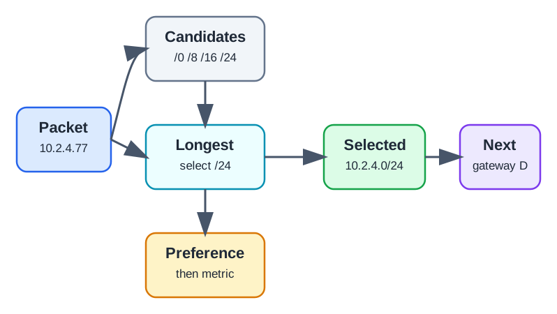
Test destinations such as 10.2.4.77, 10.2.9.12, 10.8.1.5, and 198.51.100.20. For each destination, list every matching prefix and then select the longest matching prefix.

Figure 10.1: Longest-prefix match lab: destination candidates are filtered by matching prefix length before route source or metric is considered.

Record the decision in this compact form:

• Destination: 10.2.4.77.
• Matching prefixes: /0, /8, /16, /24.
• Selected prefix: 10.2.4.0/24.
• Next hop: gateway D.
• Reason: /24 is more specific than /16, /8, and /0.
• Rejected assumption: a lower metric on the /8 route would not override the /24 match.

Acceptance standard: Your report must show the rejected candidates, not only the winning route.

10.7 Lab 2: Dijkstra Link-State Trace

Goal: Compute shortest paths from one source when the full topology is known.

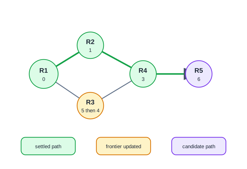
Use a five-router topology with weighted links:

• R1 to R2 has weight 1.
• R1 to R3 has weight 5.
• R2 to R4 has weight 2.
• R3 to R4 has weight 1.
• R4 to R5 has weight 3.

Start from R1. Keep three sets during the lab:

• Settled nodes: shortest path is final.
• Frontier nodes: tentative path weight is known.
• Unseen nodes: no candidate path has been found yet.

Figure 10.2: Dijkstra lab frontier: settled nodes, frontier candidates, and unseen nodes are updated until each destination has a shortest path and next hop.

Run it: Reproduce this topology in the Dijkstra workbench below and let it settle nodes for you. Enter the five routers and link weights, start from R1, and step the algorithm so you can watch the frontier grow, a node settle by lowest tentative weight, and a tentative path improve after a later step. Then remove the R1-R2 link and re-run to see which next hops change, and record the settle order and improved path the acceptance standard asks for.

Walk through the trace:

1. Mark R1 settled with weight 0.
2. Add R2 with tentative weight 1 and R3 with tentative weight 5.
3. Settle R2 because it has the lowest tentative weight.
4. Update R4 through R2 with weight 3.
5. Settle R4 before R3 because 3 is less than 5.
6. Improve R3 through R4 to weight 4.
7. Add R5 through R4 with weight 6.
8. Finish when all reachable nodes are settled.

For R1, the selected next hop for R3, R4, and R5 is R2 because the shortest known paths from R1 begin through R2. If the R1-R2 link is removed, rerun the trace and document which next hops change.

Acceptance standard: Your report must include at least one tentative path that was improved after a later step.

10.8 Lab 3: Distance-Vector Rounds

Goal: Observe convergence when routers only exchange neighbor distance information.

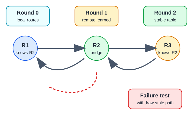
Use a simple chain: R1 connected to R2, and R2 connected to R3. Each direct link has weight 1. Begin with each router knowing only itself and directly connected neighbors.

Run it: Watch the rounds play out in the DSDV distance-vector workbench below. Build the R1-R2-R3 chain, then step the rounds and watch each router’s table fill in as neighbors advertise their distances, until no entry changes and the network has converged. Break the R2-R3 link and watch how stale routes linger and how split horizon or poisoned reverse withdraws them, then record which entries went invalid and how they were cleared.

Run update rounds:

1. Round 0: each router knows only local and neighbor routes.
2. Round 1: R1 learns R3 through R2, and R3 learns R1 through R2.
3. Round 2: if no entries change, the topology has converged.

Figure 10.3: Distance-vector rounds lab: routers exchange neighbor distance information, update routes by adding link weight, and use split horizon or poison reverse to reduce loops.

Then test a failure:

• Remove the R2-R3 link.
• Identify which entries become invalid.
• Record whether R1 keeps stale information about R3.
• Apply split horizon or poison reverse in the model.
• Show how the invalid route is withdrawn or marked unreachable.

Do not state that distance-vector behavior is always slow or always unstable. The observed behavior depends on timers, triggered updates, maximum metric, route poisoning, topology, and implementation details.

Acceptance standard: Your report must separate the algorithmic rule from protocol-specific timer behavior.

10.9 Algorithm Comparison

Use this comparison during the lab check:

• Longest-prefix match is a forwarding lookup rule. It chooses a route entry for a destination address.
• Dijkstra-style computation is used by link-state routing after a router has topology information.
• Bellman-Ford-style updates are used by distance-vector systems that learn through neighbor reports.
• RPL is not simply RIP or OSPF for small devices. It uses DODAG structure, Rank, Objective Functions, Trickle timers, and parent selection rules for low-power and lossy IPv6 networks.

The practical check question is not “which algorithm is best?” The useful question is “which records does this algorithm require, and what failure mode does it create if those records are stale, incomplete, or too expensive to maintain?”

10.10 Verification Checklist

Before marking the algorithm lab complete, confirm that you have:

• Listed all matching prefixes for at least one lookup.
• Shown why the default route loses when a more specific route matches.
• Traced at least four Dijkstra steps from source to final path.
• Recorded one tentative path that improves during the Dijkstra trace.
• Shown at least two distance-vector update rounds.
• Tested one route withdrawal or link removal.
• Named the loop-control technique used in the distance-vector lab.
• Explained why RPL objective-function records are a separate constrained-network design question.

10.11 Common Mistakes

• Comparing route metrics before checking longest-prefix match.
• Treating Dijkstra output as a packet trace rather than a route computation.
• Assuming every link-state protocol has identical timers, areas, and policy behavior.
• Treating split horizon as a complete guarantee that loops cannot happen.
• Saying that RPL is just distance-vector routing with a different name.
• Reporting only the final path without showing the rejected candidates.

10.12 Knowledge Check

10.13 Matching Quiz

10.14 Ordering Quiz

10.15 Summary

Routing algorithm labs should make decisions visible. Longest-prefix match proves which route entry a packet uses. Dijkstra-style tracing proves how link-state computation chooses next hops from topology records. Distance-vector rounds prove how neighbor reports converge and how stale routes can be reduced with split horizon or poison reverse. For constrained IoT networks, connect these ideas to RPL carefully: parent selection, Rank, Objective Functions, and Trickle behavior are not interchangeable with generic enterprise routing assumptions.

10.16 Key Takeaway

Routing algorithm labs should connect table traces to field deployment behavior: convergence, loop prevention, route choice, and failure recovery must be explained with operational records.

10.17 Concept Relationships

• Routing Labs: Advanced explains the routing-record structure used here.
• Routing Tables and Route Types provides route lookup and longest-prefix mechanics.
• Packet Switching and Failover connects route changes to packet movement.
• RPL Core Concepts continues into DODAG and Rank behavior.
• RPL Fundamentals connects objective functions to constrained-network routing.

10.18 What’s Next

Continue to Routing Labs: Fundamentals if you need more command-level lab-record practice, or move to Routing Labs and Quiz to check the lab sequence before starting the RPL-specific chapters.