5  Diagnosing IoT Architecture Anti-Patterns

5.1 Start With the Symptom on the Floor

The story starts when an architecture that looked simple begins to misbehave: cloud bills climb, dashboards break after a sensor change, or relay nodes near the gateway lose battery first.

Use the reference model as a flashlight for missing work. Find the layer that should own buffering, filtering, abstraction, local control, or routing balance before you pick an architecture label.

In 60 Seconds

Reference models help teams find missing responsibilities before they become production failures. The three anti-patterns to catch early are cloud-only pipelines, direct database access from applications, and energy-hotspot routing. The fix is not “add more layers”; it is to place edge processing, data accumulation, abstraction, applications, and human workflows where the latency, cost, reliability, and governance constraints require them.

Minimum Viable Understanding

• Three common anti-patterns cause most IoT architecture failures: cloud-only (missing edge processing), direct database access (missing abstraction), and energy hotspots (unbalanced load).
• Layer placement is a design decision: keep time-critical control close to devices, buffer and normalize data before it reaches cloud services, and expose applications through stable APIs instead of storage schemas.
• Most production IoT systems are hybrid: use the architecture decision tree to identify the dominant pattern, then combine edge, fog, cloud, and mesh approaches where the workload demands it.

Chapter Roadmap

1. First use the reference model to find the missing responsibility behind a visible symptom.
2. Then test the three recurring anti-patterns: cloud-only ingest, direct database access, and energy-hotspot routing.
3. Next compare smart-home, warehouse, grid, and architecture-selection scenarios so the same layer vocabulary works across domains.
4. After that pressure-test the numbers with the edge-versus-cloud cost example and calculator.
5. Finally close with pitfalls, quizzes, concept links, and next design-pattern chapters.

Checkpoint callouts recap the path; collapsed visuals, scenarios, calculators, and quizzes support a deeper pass.

5.2 Use the Model to Find Missing Work

A reference model is useful when it reveals a responsibility that has nowhere to live. The broken design usually looks simple because one layer is doing another layer’s work. In IoT, that missing work often sits between the physical device and the user-facing application: filtering raw telemetry, buffering during outages, translating device-specific payloads, enforcing command contracts, or keeping local safety behavior alive when the cloud path is unavailable.

The anti-pattern is not “too few boxes on a diagram.” It is a responsibility mismatch. A cold-chain gateway that forwards every DS18B20 or SHT31 reading to a cloud database without local threshold checks has made the cloud responsible for bandwidth, latency, and outage recovery. A dashboard that queries PostgreSQL, TimescaleDB, or InfluxDB tables directly has made the application responsible for storage schema changes. A mesh network that routes all traffic through nodes near one LoRaWAN, Zigbee, or Thread border router has made battery-powered relays responsible for traffic they cannot sustain.

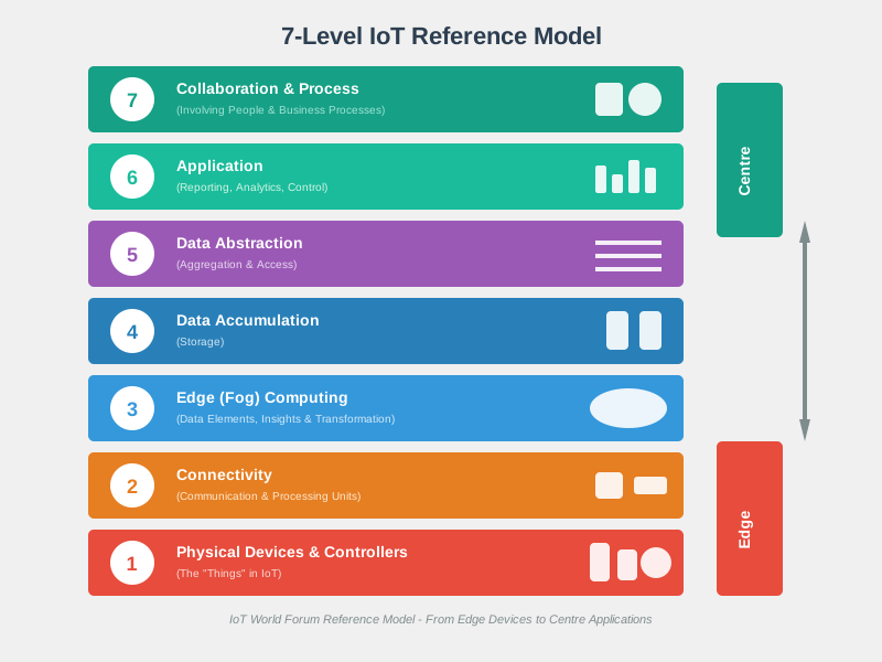
The reference model gives the review a shared vocabulary. Layer 1 device behavior includes sensing, actuation, calibration, and power. Layer 2 covers connectivity such as Wi-Fi, BLE, Ethernet, LTE-M, LoRaWAN, Zigbee, Thread, or Modbus. Layer 3 edge processing handles local thresholds, filtering, aggregation, protocol adaptation, and safe fallback. Layer 4 accumulation stores events, windows, and histories. Layer 5 abstraction exposes stable APIs and units. Layers 6 and 7 turn those capabilities into applications and human workflows.

A good diagnosis asks where the failing responsibility belongs before choosing a pattern label. Edge, fog, cloud, mesh, and hybrid architectures are outcomes of that placement decision, not slogans. Most production systems combine them: the device or gateway handles local control, a broker such as Mosquitto, EMQX, or AWS IoT Core handles message movement, a time-series store keeps history, and an API or domain service protects applications from raw device schemas. The model is useful when it makes those boundaries explicit enough to test.

5.3 Diagnose the Symptom Before Choosing the Pattern

Map the failure symptom to the missing layer responsibility before changing the topology. Start with the observed failure, then collect one measurement that proves where the pressure is. A warehouse deployment with rising cloud costs needs message rate, payload size, drop rate, and rollup ratio before anyone adds a new cloud service. A smart-building dashboard that breaks after adding BACnet or Modbus devices needs evidence of schema coupling, unit conversion, and API ownership. A battery mesh that loses nodes near a gateway needs relay count, retransmission count, duty cycle, and current draw.

• High latency or outage sensitivity: add edge processing for local thresholds, aggregation, and safe fallback before cloud services.
• Apps breaking when data changes: add an API or domain service boundary instead of letting user interfaces query storage schemas directly.
• Uneven battery drain or overloaded relays: rebalance routing, duty cycle, gateway placement, and forwarding policy near the network layer.

Then write the smallest boundary change that addresses the evidence. For a freezer-monitoring fleet, that may be an edge rule on a Raspberry Pi, industrial gateway, AWS IoT Greengrass component, or Azure IoT Edge module that sends only threshold events and periodic summaries to the cloud. For an analytics portal, it may be a /v1/devices/{id}/readings API that normalizes Celsius/Fahrenheit, sensor quality flags, and time windows before data reaches Grafana, a React dashboard, or a mobile app. For a mesh, it may be additional gateways, parent selection rules, reporting intervals, or local aggregation.

Review the redesign against operating conditions. Disconnect the WAN and verify which functions continue locally. Add a new sensor vendor and verify the application sees the same resource and unit contract. Replay a traffic burst and verify the broker, queue, and database stay within latency and retention limits. If the symptom moves to a different layer, stop and update the model instead of forcing the original diagnosis. The best pattern is the one whose boundaries still make sense after scale, outage, schema change, and support handoff are tested.

5.4 Why Anti-Patterns Survive Early Demos

Architecture anti-patterns often pass early tests because scale, outage, firmware diversity, and operational handoff are absent. Ten sensors can hide a cloud-only design. One dashboard can hide direct database coupling. A short indoor demo can hide a mesh energy hotspot. The demo path exercises the happy path; the reference model review asks whether each layer still has a clear contract when the path is stressed.

flowchart TD
  A[Observed symptom] --> B{Which responsibility is missing?}
  B -->|Raw volume, latency, outage| C[L3 edge filtering and local fallback]
  B -->|Schema or unit coupling| D[L5 API and domain abstraction]
  B -->|Relay drain or retransmits| E[L1-L2 power and routing review]
  C --> F[Measure message rate, rollup ratio, and backhaul loss]
  D --> G[Measure client schema dependencies and unit mappings]
  E --> H[Measure duty cycle, retries, RSSI, and parent load]
  F --> I[Move the smallest boundary]
  G --> I
  H --> I
  I --> J[Test scale, outage, schema change, and handoff]

Reference-model diagnosis loop for mapping symptoms to layer responsibilities before selecting an architecture pattern.

The deeper mechanism is coupling. A cloud-only design couples device behavior to backhaul availability and cloud latency. Direct database access couples applications to table names, column units, retention policy, and storage engine choices. Energy-hotspot routing couples network lifetime to a few relay nodes. Each coupling may be invisible in a pilot because the dataset is small, the field network is clean, and the same engineer owns device code, backend, and dashboard.

Use the model to make coupling measurable. Count how many application files know vendor table names. Count how many commands require cloud round trips before a local actuator can fail safe. Count how many packets a relay forwards compared with the average node. Track p95 end-to-end latency, broker queue depth, time-series write rate, gateway disk retention, and reconnect behavior after a WAN outage. These signals tell the team whether the system needs edge filtering, a protocol bridge, a queue, an API abstraction, another gateway, or simply a tighter operational limit.

The model should also drive the launch test. A mature design can explain which layer owns calibration, identity, buffering, normalization, command state, dashboard queries, and support escalation. It can survive adding a new firmware version, a new sensor vendor, a temporary cloud outage, and a traffic burst without every layer learning every other layer’s internals. If the answer depends on one layer silently absorbing every responsibility, the architecture needs a boundary before launch.

Checkpoint: Diagnosis Loop

You now know:

• Start with a symptom and collect one measurement that proves where the pressure sits.
• Layer 3 handles edge processing, Layer 4 accumulates histories, Layer 5 abstracts stable APIs and units, and Layers 6-7 turn those contracts into applications and workflows.
• A launch review should test scale, outage, schema change, and support handoff before naming the final pattern.

Sensor Squad: Learning from Mistakes

Max the Microcontroller once tried to build an IoT system the “easy” way – he sent ALL of Sammy’s sensor data straight to the cloud, skipping local processing entirely.

“It worked great with 10 sensors!” Max said proudly. But when the system grew to 1,000 sensors, Bella the Battery was exhausted, the cloud bill was enormous, and everything crashed during an internet outage.

Lila the LED asked, “Why not have a helper nearby?” That helper is an edge gateway – like a teacher’s assistant who handles simple questions locally so the head teacher (the cloud) only deals with the important stuff.

Sammy the Sensor learned the lesson: “Skipping steps might seem simpler at first, but it creates bigger problems later. The 7-layer model exists for a reason!”

5.5 Learning Objectives

By the end of this chapter, you will be able to:

• Diagnose anti-patterns: Detect cloud-only, direct-database, and energy-hotspot architectural mistakes from system symptoms
• Prescribe solutions: Redesign faulty architectures by inserting the correct processing, abstraction, or routing layers
• Evaluate scenarios: Extract architecture lessons from warehouse, smart-grid, fleet, and smart-home deployment scenarios without copying vendor-specific topology blindly
• Apply decision frameworks: Select dominant architecture patterns using the architecture decision tree for new projects
• Troubleshoot systematically: Isolate IoT failures by mapping symptoms to specific reference-model layers

For Beginners: What Is an Anti-Pattern?

An anti-pattern is a common solution that looks right but actually causes problems. Think of it as a “trap” that many teams fall into:

• Cloud-only trap: Sending all data to the cloud seems simple, but it creates huge costs and fails when the internet goes down.
• No abstraction trap: Letting apps talk directly to databases seems faster, but it breaks everything when you add new sensor types.
• Energy hotspot trap: Routing all traffic through one gateway seems efficient, but it drains batteries near that gateway.

Learning to recognize these mistakes saves months of debugging and thousands of dollars in production.

5.6 Common Architecture Anti-Patterns and Solutions

~15 min | Advanced | P04.C18.U03

With the diagnosis loop in place, recognize the shortcut that created the pressure. These anti-patterns look efficient during a pilot and become expensive when scale, outage, or device diversity arrives.

Understanding what NOT to do is as important as best practices. Here are frequent mistakes in IoT reference architecture implementation:

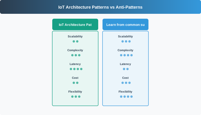
Figure 5.1: IoT architecture patterns versus anti-patterns, comparing correct layered designs with brittle shortcuts

Use the comparison in Figure 5.1 as a review lens: a pattern is useful only when it places the right responsibility at the right layer, while an anti-pattern hides a missing edge, data, API, or operations boundary until the system is stressed.

5.6.1 Anti-Pattern 1: Cloud-Only Architecture (Skipping Layers 3-5)

Problem:

Sensors (L1) → Wi-Fi (L2) → Cloud (L6-L7)

• 1000 sensors x 1 reading/second = 1000 msgs/sec to cloud
• Bandwidth cost: $5,000/month on cellular
• Latency: 200-500ms round-trip prevents real-time control
• Reliability: Internet outage = complete system failure

Solution:

Sensors (L1) → Wi-Fi (L2) → Edge Gateway (L3) → Database (L4) →
API (L5) → Apps (L6) → Users (L7)

• L3 filters 1000 msgs/sec → 50 msgs/sec (20x reduction)
• L4 stores locally, syncs summaries to cloud
• L5 abstracts sensor types from applications
• Result: $5K/month → $200/month, <10ms local response, offline operation

5.6.2 Anti-Pattern 2: Direct Database Access from Applications (No Layer 5)

Problem:

Dashboard queries PostgreSQL directly:
SELECT * FROM sensor_readings WHERE sensor_id = 'zigbee_042'

• Adding LoRaWAN sensors breaks dashboard (different table schema)
• Temperature in Celsius (Zigbee) vs Fahrenheit (legacy sensors) = manual conversion
• No access control granularity (all apps see all data)

Solution (Layer 5 Abstraction):

Dashboard calls: GET /api/sensors/042/temperature?unit=celsius
Layer 5 API:
1. Translates sensor_id to correct backend (Zigbee table, LoRaWAN table)
2. Converts units if needed
3. Enforces access controls
4. Returns: {"sensor": "042", "temperature": 25.5, "unit": "celsius"}

• Result: Add new sensor types without changing apps, centralized unit conversion

5.6.3 Anti-Pattern 3: Hotspot Energy Depletion (WSN/M2M)

Problem:

100 sensors → 1 gateway (single path)
Sensors near gateway relay 90% of traffic → batteries die in 3 months
Edge sensors still have 95% battery but network is disconnected

Solution:

100 sensors → 3 gateways (distributed load)
Each gateway handles ~33 sensors
Energy consumption balanced across network

• Result: 3-month lifetime → 2-year lifetime, same battery capacity

5.6.4 Troubleshooting Guide by Layer

5.6.4.1 High cloud costs

Likely layerL3 missing or too thin DiagnosticMeasure messages per second forwarded to cloud services. FixAdd edge filtering, local aggregation, and event-only forwarding.

5.6.4.2 Slow dashboard

Likely layerL4 accumulation problem DiagnosticCheck query time, indexing, retention policy, and write volume. FixUse a time-series store, indexes, rollups, or hot/cold storage tiers.

5.6.4.3 Cannot add new sensors

Likely layerL5 abstraction missing DiagnosticLook for application code that knows vendor tables, units, or protocol payloads. FixAdd an API or canonical event model between devices and applications.

5.6.4.4 Works online, fails offline

Likely layerL3 autonomy too weak DiagnosticDisconnect cloud backhaul and test which decisions still execute locally. FixMove safety rules, buffering, and essential control loops to edge or fog.

5.6.4.5 Battery dies fast

Likely layerL1-L2 power and routing DiagnosticProfile duty cycle, retransmissions, and relay load near gateways. FixUse duty cycling, balanced routing, adaptive reporting, or more gateways.

Try It: Layer Symptom Triage

For one IoT system you have seen or designed, write a three-row triage note before proposing a fix:

Symptom	Layer to inspect first	Evidence to collect
Cloud bill or dashboard latency is rising	L3 edge processing and L4 accumulation	Messages per second forwarded, rollup ratio, query latency, retention policy
New device types break existing applications	L5 data abstraction and API contract	Application code that names vendor tables, unit-conversion rules, schema-change history
Outages stop local safety or comfort functions	L3 local autonomy and L2 connectivity	Backhaul-disconnect test result, buffered command behavior, local control-loop log

Only commit to a redesign after each symptom has one measured signal. If the evidence points to different layers, treat the system as hybrid rather than forcing a single pattern.

Checkpoint: Anti-Patterns

You now know:

• Cloud-only designs can push 1000 messages per second to the cloud and turn a pilot into a cost and outage problem.
• Edge filtering can reduce 1000 messages per second to 50, cutting the example from $5K/month to $200/month while restoring local response.
• Direct database access points to missing Layer 5 abstraction; energy-hotspot routing points to unbalanced L1-L2 power and forwarding load.

Knowledge Check: Scalability Anti-Patterns

5.7 Architecture Scenarios

~20 min | Intermediate | P04.C18.U04

Trust the anti-pattern checklist by applying it to concrete systems. Each scenario asks which layer should own local control, buffering, abstraction, analytics, and operations handoff.

5.7.1 Smart Home IoT Topology and Power Architecture

Before moving to larger systems, examine a concrete smart home deployment that illustrates the 7-level reference model in a residential context.

This diagram reveals several key architectural patterns that map to the 7-level reference model:

Level 1 (Physical Devices):

• Battery-powered sensors: Motion detectors, door/window sensors (3-5 year battery life)
• Mains-powered actuators: Smart lights, thermostats, door locks (continuous power via PoE or AC)
• PoE-enabled devices: IP cameras, access control panels (receive both data and power via single Ethernet cable)

Level 2 (Connectivity):

• Star topology with central hub: Zigbee coordinator or Z-Wave controller acts as network center
• Power-over-Ethernet (PoE): IEEE 802.3af/at injectors provide up to 25.5W per device, eliminating need for separate power wiring
• Communication range: Zigbee mesh extends effective range; PoE supports 100m cable runs

Level 3 (Edge Computing):

• Gateway performs: Protocol translation (Zigbee to Wi-Fi), rule-based automation (“turn on lights when motion detected after sunset”), local device pairing/management
• Offline operation: Critical functions (unlock door, emergency lighting) work without internet

Architectural Benefits:

5.7.1.1 PoE infrastructure

Single cable for data and power reduces retrofit complexity for mains-powered devices.

Model mappingL1 physical devices plus L2 connectivity

5.7.1.2 Star topology

Hub failure is easy to identify and device faults are isolated from other spokes.

Model mappingL2 connectivity

5.7.1.3 Mixed power sources

Battery sensors can keep reporting during outages while PoE devices support higher-power tasks.

Model mappingL1 physical devices

5.7.1.4 Local gateway

Motion-to-light automation can run locally without waiting for cloud round trips.

Model mappingL3 edge computing

Real-World Example: Retrofit Installation Cost Analysis

For a 3-bedroom home (25 devices total):

Traditional AC Wiring Approach:

• Electrician labor: $150/outlet x 15 AC outlets = $2,250
• Materials (outlets, wiring): $500
• Total: $2,750

PoE + Battery Hybrid Approach:

• 1x PoE switch (8-port): $120
• 10x PoE devices (lights, locks, thermostats): $0 additional wiring
• 15x battery-powered sensors: $0 wiring
• Total: $120 (98% cost reduction for wiring infrastructure)

This smart home architecture demonstrates how thoughtful application of the 7-level reference model - particularly optimizing Levels 1-3 (devices, connectivity, edge) - can reduce deployment complexity while improving system reliability through local processing and mixed power architectures.

Scenario: Automated Warehouse Using the 7-Level Model

Industry: Logistics and fulfillment operations

Challenge: A warehouse automation team has mobile robots, conveyors, scanners, environmental sensors, and human safety zones. Early pilots connect each subsystem directly to a central application. The result is brittle integration, high latency for local safety decisions, and duplicated device-specific logic across dashboards.

Solution Architecture (Mapped to 7-Level Model):

Level 1 (Physical Devices): - Autonomous mobile robots, conveyor sensors, barcode scanners, robotic arms, and environmental sensors - Safety devices such as light curtains, emergency stops, and human-presence sensors

Level 2 (Connectivity): - Wired Ethernet for fixed conveyors and scanners where predictable bandwidth matters - Industrial Wi-Fi or private wireless for mobile robots and yard operations - Separate safety network or safety-rated control path where required

Level 3 (Edge Computing): - Zone controllers handle robot coordination, conveyor jam detection, and local routing decisions - Safety and motion decisions stay local because cloud round trips are too slow and too failure-prone - Edge nodes buffer events when the cloud link is unavailable

Level 4 (Data Accumulation): - Local operational store for current package locations, robot status, and conveyor state - Time-series store for equipment telemetry and maintenance signals - Cloud storage for long-term analytics and cross-site learning

Level 5 (Data Abstraction): Unified device API - Standard device-state endpoint, such as /api/devices/{id}/state, regardless of vendor - Adapters convert robot, conveyor, and scanner formats into a canonical event model - Applications consume stable APIs rather than vendor schemas

Level 6 (Application): Warehouse management systems - Package tracking dashboard - Predictive maintenance application - Human work-assignment and safety-monitoring tools - Energy and utilization reporting

Level 7 (Collaboration & Processes): Human-machine coordination - Operations teams respond to throughput and safety alerts - Maintenance teams service equipment based on telemetry trends - Site teams share validated rules and dashboards across facilities

Expected results:

• Lower latency: local controllers make safety and routing decisions without cloud dependency
• Cleaner integration: new equipment requires an adapter, not a dashboard rewrite
• Better resilience: operations can continue in degraded mode during backhaul outages
• Clear ownership: controls engineers own L1-L3, platform teams own L4-L5, application teams own L6, operations owns L7

Lessons Learned:

• Do not send safety-critical control loops to the cloud.
• Do not expose vendor-specific tables or payloads directly to applications.
• Use the reference model to clarify responsibility boundaries, not to force seven separate physical platforms.

Scenario: Smart Grid Monitoring Using an IoT-A Style Model

Industry: Energy (electrical grid management)

Challenge: A utility has smart meters, feeder sensors, transformers, substations, and customer-facing applications. Multiple device vendors and regulatory environments make direct device-to-application integration expensive and difficult to govern.

Solution Architecture (Mapped to IoT-A Reference Model):

Resource Layer: Physical grid assets - Smart meters, power-quality sensors, transformers, substations, and automated switching equipment

IoT Service Layer: Standardized device services - Meter-reading service, power-quality service, asset-health service, and control service - Protocol adapters normalize vendor data into service contracts

Virtual Entity Layer: Digital twins of grid assets (IoT-A’s unique contribution) - Each transformer represented as virtual entity with properties: location, capacity, temperature, load, health_status - Virtual entity aggregates data from multiple physical sensors (oil temperature, bushing current, tap changer position) - Digital twin enables “what-if” simulations: “If transformer T-4521 fails, which transformers will be overloaded?”

Service Organization Layer: Orchestrated grid services - Load balancing service: Monitors all transformers, triggers automatic load shedding if overload detected - Outage detection service: Correlates smart meter connectivity loss patterns to identify grid failures - Renewable integration service: Coordinates solar/wind fluctuations with grid storage and demand response

Application Layer: Utility operations - Grid operations dashboard - Predictive maintenance app - Customer billing app integrating smart meter data with CRM and invoicing systems - Regulatory reporting app

Business Layer: Strategic grid management - Revenue protection: Detect energy theft through anomaly detection - Capital planning: Use digital twin simulations to optimize grid expansion investments - Renewable integration: Maximize solar/wind usage while maintaining grid stability

Cross-Cutting Security and Governance: - Privacy controls before analytics - Encryption and device identity across telemetry paths - Role-based access control for field, operations, and executive views

Expected results:

• Interoperability: service contracts reduce vendor-specific application code
• Digital twin value: virtual entities allow analysis by asset, not just by sensor stream
• Outage response: correlated readings help locate faults faster than isolated alarms
• Governance: privacy and access controls are applied consistently across services

Lessons Learned:

• IoT-A’s virtual entity layer is powerful for physical infrastructure digital twins - transformers, substations represented as software objects
• Service organization layer critical for complex orchestration (load balancing requires coordinating meters, sensors, substations simultaneously)
• Business layer alignment keeps IoT investment tied to reliability, resilience, and regulatory goals rather than technology experiments
• Cross-cutting governance is easier to maintain than per-layer security bolt-ons

5.8 Architecture Selection Decision Tree

After the scenarios, switch from diagnosis to selection. Pattern names come after latency, scale, connectivity, environment, and ownership evidence.

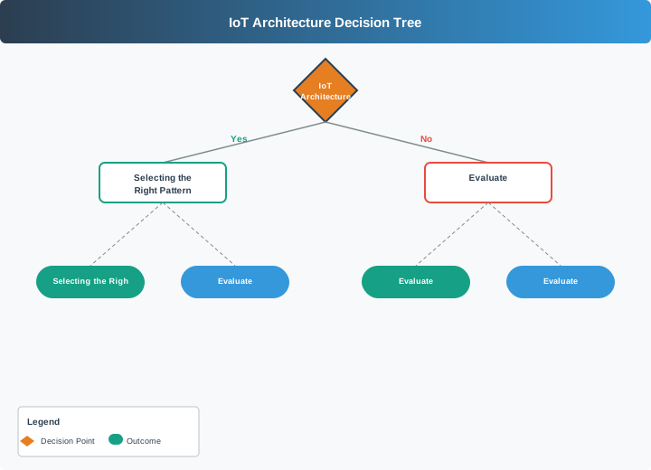
When designing an IoT system, choosing the right architecture pattern is critical. Use this decision tree to guide your selection:

Figure 5.2: IoT Architecture Decision Tree: Selecting the Right Pattern

5.8.1 Quick Architecture Comparison

5.8.1.1 Edge

Best for: real-time control and privacy.

LatencyUsually under 50 ms ScaleLow to medium per node ConnectivityLocal first ComplexityHigh

5.8.1.2 Fog

Best for: site or regional aggregation.

LatencyRoughly 50-500 ms ScaleMedium to high ConnectivityRegional ComplexityMedium-high

5.8.1.3 Cloud

Best for: analytics, storage, and fleet management.

LatencyOften 100 ms to seconds ScaleVery high ConnectivityRequires backhaul ComplexityMedium

5.8.1.4 WSN

Best for: environmental sensing and mesh coverage.

LatencyVaries by duty cycle and route ScaleVery high when planned well ConnectivityMesh or clustered ComplexityHigh

5.8.1.5 M2M

Best for: direct device coordination.

LatencyOften under 100 ms locally ScaleMedium ConnectivityPeer-to-peer or local broker ComplexityMedium

5.8.1.6 Hybrid

Best for: most real deployments.

LatencyVaries by workload ScaleHigh ConnectivityMixed local and cloud paths ComplexityHigh but manageable with clear boundaries

Practical Advice: Most Systems Are Hybrid

Real-world IoT systems rarely use a single architecture pattern. A smart factory might use:

• Edge: Safety interlocks (must react in <10ms)
• Fog: Quality control aggregation (per-line statistics)
• Cloud: Production analytics, ML model training
• M2M: Robot-to-robot coordination on the floor

The decision tree helps you identify the dominant pattern, but plan for hybrid architectures as your system matures.

Knowledge Check: Architecture Selection

Checkpoint: Pattern Selection

You now know:

• Edge is the first place to look for real-time control, privacy, bandwidth limits, or offline reliability.
• Fog fits regional aggregation and 10-50 ms site decisions; cloud fits long-term storage, fleet dashboards, ML training, and business processes.
• A sparse 10,000-acre farm with one reading every 15 minutes is not a cloud-only problem when cellular coverage is unreliable.

5.9 Visual Reference Gallery

Use the gallery as a visual cross-check before the math-heavy section: the same layer names should still explain data flow and handoff boundaries.

Visual: 7-Level IoT Reference Model

Figure 5.3: Cisco 7-level IoT reference model architecture

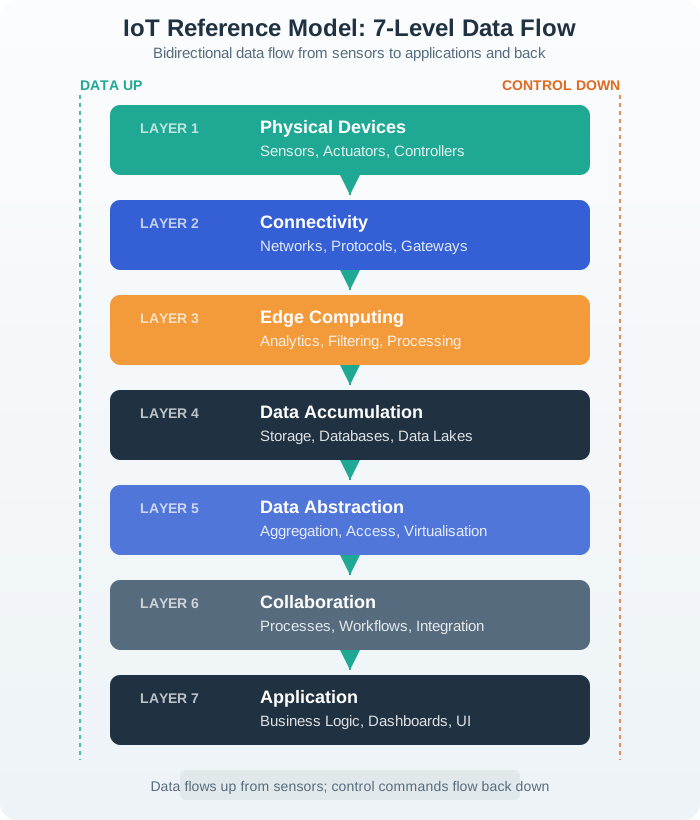
Visual: IoT Reference Model Data Flow

Figure 5.4: Data flow through 7-level architecture

Visual: Comparing Reference Models

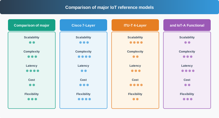
Figure 5.5: Comparison of major IoT reference models

Worked Example: Calculating Edge Processing Bandwidth Savings for Smart City Deployment

Scenario: A smart city deploys 10,000 environmental sensors (temperature, humidity, air quality, noise) reporting every 30 seconds. Calculate bandwidth and cloud costs for cloud-only vs edge-processing architectures.

Given Data:

• 10,000 sensors across the city
• Reporting interval: 30 seconds
• Payload per reading: 250 bytes (JSON: sensor ID, timestamp, 4 measurements + metadata)
• Cellular data cost: $0.10/MB
• Cloud processing cost: $0.000002 per message (AWS IoT Core)
• Edge gateway: $500 each, processes 500 sensors, filters/aggregates data

Architecture 1: Cloud-Only (No Edge Processing)

Step 1: Calculate Message Rate

• Messages per hour: 10,000 sensors × (3,600s / 30s) = 10,000 × 120 = 1,200,000 messages/hour
• Messages per month: 1,200,000 × 24 × 30 = 864,000,000 messages/month

Step 2: Calculate Bandwidth

• Data per month: 864M messages × 250 bytes = 216,000 MB = 216 GB/month
• Bandwidth cost: 216 GB × 1,000 MB/GB × $0.10/MB = $21,600/month

Step 3: Calculate Cloud Processing Cost

• Processing cost: 864M messages × $0.000002 = $1,728/month

Total Cloud-Only Cost: $21,600 + $1,728 = $23,328/month

---

Architecture 2: Edge Processing with Aggregation

Edge gateways perform local processing: - Filter: Remove duplicate readings (sensors report unchanged values → drop 40% of messages) - Aggregate: Send zone averages every 5 minutes instead of per-sensor readings (10x reduction) - Anomaly alerts: Forward only readings outside normal ranges (5% of total)

Step 1: Calculate Effective Message Reduction

• Original: 1,200,000 messages/hour
• After filtering (40% removed): 1,200,000 × 0.6 = 720,000 messages/hour
• Zone aggregation: 10,000 sensors ÷ 100 sensors per zone = 100 zones; 100 zones × (3,600s / 300s) = 1,200 aggregate messages/hour (600x reduction for normal data)
• Anomaly alerts (5% of filtered): 720,000 × 0.05 = 36,000 messages/hour

Total messages to cloud: 1,200 (aggregates) + 36,000 (alerts) = 37,200 messages/hour - Monthly: 37,200 × 24 × 30 = 26,784,000 messages/month (97% reduction vs cloud-only)

Step 2: Calculate Bandwidth

• Aggregates: 1,200 msg/hr × 150 bytes (smaller payload) × 24 × 30 = 129.6 MB/month
• Alerts: 36,000 msg/hr × 250 bytes × 24 × 30 = 6,480 MB/month
• Total bandwidth: 6,609.6 MB = 6.45 GB/month (97% reduction)
• Bandwidth cost: 6.61 GB × 1,000 MB/GB × $0.10/MB = $661/month

Step 3: Calculate Cloud Processing Cost

• Processing cost: 26.78M messages × $0.000002 = $54/month

Step 4: Calculate Edge Infrastructure Cost

• Gateways needed: 10,000 sensors ÷ 500 per gateway = 20 gateways
• Gateway cost: 20 × $500 = $10,000 (one-time)
• Amortized over 3 years: $10,000 ÷ 36 months = $278/month

Total Edge Architecture Cost: $661 + $54 + $278 = $993/month

---

Comparison Summary:

5.9.0.1 Cloud-only baseline

Monthly cost$23,328 Bandwidth216 GB Messages to cloud864 million per month SavingsBaseline

5.9.0.2 Edge processing

Monthly cost$993 Bandwidth6.45 GB Messages to cloud26.8 million per month Savings$22,335 per month, about 96%

Payback Period: $10,000 gateway investment ÷ $22,335 monthly savings = 0.45 months (13 days)

Decision: Deploy edge gateways with local filtering and aggregation. The 96% cost reduction and 13-day payback make edge processing a clear winner. Additionally, edge processing provides local resilience (sensors continue reporting locally during internet outages).

Putting numbers to it: Edge savings scale with device count, reporting rate, message reduction, and gateway amortization. In this example, 10,000 sensors reporting 120 times per hour drop from 864 million cloud messages per month to 26.8 million after edge filtering and aggregation, saving about $22,335 per month before considering resilience benefits.

Checkpoint: Cost Signals

You now know:

• The smart-city example starts at 864 million cloud messages per month and 216 GB/month of data.
• Edge filtering and aggregation reduce that to 26.8 million cloud messages, 6.45 GB/month, and about $22,335/month in savings.
• The example gateway investment is $10,000, amortized to $278/month, with a 13-day payback signal.

Try It: Edge vs Cloud Cost Calculator

Adjust the deployment parameters to explore how edge processing affects monthly costs compared to cloud-only architecture.

viewof epSensors = Inputs.range([1000, 100000], {value: 10000, step: 1000, label: "Number of sensors"})
viewof epInterval = Inputs.range([5, 300], {value: 30, step: 5, label: "Reporting interval (sec)"})
viewof epPayload = Inputs.range([50, 1000], {value: 250, step: 50, label: "Payload size (bytes)"})
viewof epCellCost = Inputs.range([0.01, 1.0], {value: 0.10, step: 0.01, label: "Cellular cost ($/MB)"})
viewof epReduction = Inputs.range([50, 99], {value: 97, step: 1, label: "Edge message reduction (%)"})
viewof epGwCost = Inputs.range([100, 2000], {value: 500, step: 100, label: "Gateway cost ($)"})
viewof epGwCapacity = Inputs.range([100, 2000], {value: 500, step: 100, label: "Sensors per gateway"})

epCalc = {
  let msgsPerHour = epSensors * (3600 / epInterval);
  let msgsPerMonth = msgsPerHour * 24 * 30;
  let cloudBwMB = (msgsPerMonth * epPayload) / (1000 * 1000);
  let cloudBwCost = cloudBwMB * epCellCost;
  let cloudProcCost = msgsPerMonth * 0.000002;
  let cloudTotal = cloudBwCost + cloudProcCost;
  let edgeMsgsMonth = msgsPerMonth * (1 - epReduction / 100);
  let edgeBwMB = (edgeMsgsMonth * epPayload) / (1000 * 1000);
  let edgeBwCost = edgeBwMB * epCellCost;
  let edgeProcCost = edgeMsgsMonth * 0.000002;
  let numGateways = Math.ceil(epSensors / epGwCapacity);
  let gwMonthly = (numGateways * epGwCost) / 36;
  let edgeTotal = edgeBwCost + edgeProcCost + gwMonthly;
  let savings = cloudTotal - edgeTotal;
  let savingsPct = ((savings / cloudTotal) * 100);
  let paybackDays = (numGateways * epGwCost) / (savings) * 30;
  return {msgsPerMonth, cloudBwMB, cloudTotal, edgeMsgsMonth, edgeBwMB, edgeTotal, savings, savingsPct, numGateways, gwMonthly, paybackDays};
}

html`<div class="arch-result">
  <div class="arch-calculator-output">
    <div class="arch-calculator-card">
      <strong>Cloud-only</strong>
      <div>Messages/month: ${(epCalc.msgsPerMonth / 1e6).toFixed(1)}M</div>
      <div>Bandwidth: ${(epCalc.cloudBwMB / 1000).toFixed(1)} GB</div>
      <div>Monthly cost: $${epCalc.cloudTotal.toFixed(0)}</div>
    </div>
    <div class="arch-calculator-card">
      <strong>Edge processing</strong>
      <div>Messages/month: ${(epCalc.edgeMsgsMonth / 1e6).toFixed(1)}M</div>
      <div>Bandwidth: ${(epCalc.edgeBwMB / 1000).toFixed(2)} GB</div>
      <div>Monthly cost: $${epCalc.edgeTotal.toFixed(0)}</div>
    </div>
    <div class="arch-calculator-card">
      <strong>Decision signal</strong>
      <div>Monthly savings: $${epCalc.savings.toFixed(0)} (${epCalc.savingsPct.toFixed(0)}%)</div>
      <div>Gateways needed: ${epCalc.numGateways}</div>
      <div>Payback: ${epCalc.paybackDays.toFixed(0)} days</div>
    </div>
  </div>
</div>`

Decision Framework: Selecting IoT Architecture Layer Deployment

The 7-layer IoT reference model allows flexible deployment of processing across edge, fog, and cloud. This framework helps decide where each layer should run.

5.9.0.3 L1: Physical devices

Sensors and actuators must be physically present. Place sensing, actuation, and device health checks on the device.

5.9.0.4 L2: Connectivity

Connectivity spans device radios, wired links, gateways, and backhaul. Use gateways when non-IP protocols such as Zigbee, BLE, or LoRaWAN need translation.

5.9.0.5 L3: Edge computing

Deploy at device, gateway, or site edge when latency is tight, bandwidth is limited, privacy matters, or the system must keep operating offline.

5.9.0.6 L4: Data accumulation

Use cloud storage for long-term history and fleet analytics. Use fog or edge storage for short buffers, replay, and outage tolerance.

5.9.0.7 L5: Data abstraction

Use APIs, protocol adapters, and canonical data models to hide vendor payloads and storage schemas from applications.

5.9.0.8 L6: Application

Put global dashboards and analytics in the cloud. Put site-specific control apps near the site when operators need local visibility during outages.

5.9.0.9 L7: Collaboration

Business workflows, maintenance tickets, reporting, and cross-site learning usually live in cloud systems, but they depend on trustworthy lower-layer data.

Quick Selection Guide:

Deploy at Edge (Device) when:

• Real-time control (<10ms latency): safety interlocks, motor control
• Privacy-sensitive data: medical sensors, facial recognition (process locally, never send raw data)
• Bandwidth constrained: video analytics (detect events locally, send alerts only)
• Extreme reliability: must operate offline (no network dependency)

Deploy at Fog (Gateway) when:

• Regional processing (10-50ms latency): zone-level aggregation, local dashboards
• Protocol translation: multiple device protocols (LoRa, Zigbee, BLE) to IP
• Cost optimization: filter/aggregate before cloud (reduce bandwidth 90%+)
• Moderate offline resilience: buffer data during internet outages

Deploy at Cloud when:

• Long-term storage: historical data (years), regulatory compliance
• Global scale: multi-site dashboards, cross-region analytics
• ML training: large models needing GPUs
• Business processes: reporting, billing, collaboration

Hybrid Deployment Example (Smart Factory):

• L1-L2 (sensors, connectivity): On-device
• L3 (edge compute): 80% on gateway (vibration analysis, anomaly detection) + 20% on device (safety interlocks)
• L4 (data): Local DB at gateway (7 days) + cloud time-series DB (5 years)
• L5 (API): Cloud (global device access)
• L6 (apps): Factory floor dashboard at gateway + executive dashboard in cloud
• L7 (collaboration): Cloud (procurement, maintenance ticketing)

Common Mistake: Cloud-Only Architecture with High-Frequency IoT Devices

The Problem: A logistics company deployed 5,000 GPS trackers on trucks, sending location updates every 10 seconds directly to AWS IoT Core. Monthly cloud bill: $45,000 (far exceeding the $5,000 budget). Worse, during cellular dead zones, all location data was lost (no local buffering).

Why It Happens:

• “Cloud is infinitely scalable” mindset ignores per-message pricing (AWS IoT: $1/million messages + bandwidth)
• 5,000 devices × 6 updates/min × 60 min × 24 hr × 30 days = 1.296 billion messages/month
• At $1/million: $1,296/month (messaging) + $8,640/month (bandwidth @ 200 bytes/msg) = $9,936/month
• But trackers also send telemetry (speed, fuel, diagnostics) → 3x messages → $29,808/month
• Plus Lambda processing, DynamoDB writes, S3 storage → $45,000/month actual

The Correct Architecture: Edge + Fog + Cloud

Edge (Tracker Device):

• Buffer GPS readings in local flash memory (1,000 points = 12 hours @ 10s intervals)
• Detect “significant movement” (>100m from last reported position) → send update
• Static vehicles: send heartbeat every 5 minutes (not every 10 seconds)

Fog (Regional Gateway at Depot):

• When trucks return to depot, offload buffered GPS logs via Wi-Fi (free bandwidth vs cellular)
• Aggregate fleet data: “Zone 5 has 12 active trucks” instead of 12 separate messages
• Local dashboard for depot manager (no cloud latency)

Cloud (Central):

• Receive only significant events: route deviation, geofence breach, maintenance alerts
• Long-term analytics: route optimization, fuel efficiency trends
• Executive dashboard

Message Reduction:

• Original: 1.296B messages/month
• With significance filtering (90% eliminated): 130M messages/month
• With aggregation (5:1 reduction): 26M messages/month
• New cost: 26M × ($1/M) + bandwidth reduction = $1,800/month (96% savings)

Additional Benefits:

• Offline resilience: 12 hours of buffered GPS in dead zones
• Reduced cellular data: $15,000/month → $800/month
• Faster depot dashboard (local data, no cloud round-trip)

Rule of Thumb: If per-device cloud cost > per-device hardware cost annually, you’ve over-centralized. A $50 tracker shouldn’t cost $100/year in cloud fees.

Cost examples solve one failure mode, but a clean bill does not prove the architecture is healthy. Use the pitfalls as a final boundary review.

Common Pitfalls

1. Mapping reference model layers to deployment tiers one-to-one

The 7-layer IoT reference model is a logical abstraction, not a deployment blueprint. Mapping each layer to a separate physical server creates unnecessary complexity. In practice, layers 1-3 often run on the same edge gateway, and layers 4-7 run across shared cloud services. Use the model to reason about data flow and security boundaries, not to prescribe infrastructure.

Key Concepts

• IoT Reference Model: A standardized layered framework (typically 7 layers from physical devices to application) that defines how data flows, where processing occurs, and where security boundaries exist in IoT systems
• Edge Processing Layer: The third layer in most IoT reference models where local compute (gateways, edge servers) filters, aggregates, and transforms raw sensor data before forwarding to cloud, reducing bandwidth by 90%+
• Abstraction Layer: Layer 5 in the IoT reference model that decouples applications from protocol-specific device interfaces, enabling new device types to be added without changing application logic
• Digital Twin: A software model synchronizing real-time state with a physical device, enabling simulation, monitoring, and control without direct device interaction – positioned at the abstraction/application boundary
• Hub-and-Spoke Topology: An IoT architecture pattern where edge nodes (spokes) aggregate local sensor data and forward to a central hub for cloud processing, matching the 7-layer reference model’s gateway tier
• Peer-to-Peer Topology: An IoT architecture where devices communicate directly without a central hub, reducing latency for local interactions but requiring distributed consensus mechanisms for coordination
• Publish-Subscribe Pattern: An architectural decoupling pattern where publishers send messages to topics without knowing subscribers, and subscribers receive messages without knowing publishers – the dominant IoT communication pattern
• Anti-Pattern: God Service: An architectural anti-pattern where a single service handles all IoT responsibilities (ingestion, processing, storage, presentation), creating a deployment bottleneck and single point of failure

2. Ignoring the abstraction layer when onboarding new device types

Connecting new device protocols (BLE, Zigbee, proprietary) directly to application logic creates tight coupling that requires application code changes for every new device type. Always implement an abstraction/normalization layer that maps diverse protocols to a canonical data model – this is Layer 5’s core purpose in the reference model.

3. Applying a single architectural pattern to heterogeneous workloads

Hub-and-spoke works well for telemetry but introduces latency for device-to-device control. Peer-to-peer reduces latency but complicates management. Publish-subscribe decouples producers from consumers but adds broker overhead. Most production IoT systems use a hybrid of patterns – define which pattern applies to which data flow based on latency, reliability, and management requirements.

Label the Diagram

Code Challenge

5.10 Summary

In this chapter, you learned:

• Three common anti-patterns: Cloud-only (missing L3), direct database access (missing L5), and energy hotspots
• Warehouse and grid scenarios: Layer 3 edge autonomy, Layer 5 abstraction, and virtual-entity modeling prevent brittle integrations and cloud-only failure modes
• Architecture decision tree: Select based on latency requirements, scale, connectivity, and environment constraints
• Hybrid reality: Production systems typically combine multiple patterns

5.11 Key Takeaway

Reference models are useful when they force explicit placement decisions. Put latency-sensitive, safety-critical, and bandwidth-heavy work close to the device, use abstraction layers to avoid brittle integrations, and expect real IoT systems to combine multiple patterns.

5.12 Knowledge Check

Quiz: Reference Model Anti-Patterns

5.13 Concept Relationships

How These Concepts Connect

Prerequisite knowledge:

• Cloud Computing - Cloud platforms host Layers 5-7 in the 7-layer model
• Edge Computing - Edge processing implements Layer 3 data reduction

Related concepts:

• MQTT Protocol - Messaging for Layer 3-5 communication in IoT-A architecture
• Database Design - Layer 4 data accumulation storage strategies

This enables:

• Microservices Architecture - Service decomposition follows reference model layers
• System Integration - Layer 5 abstraction enables protocol translation

5.14 See Also

Related Resources

Architectural frameworks:

• ITU-T Y.4000/Y.2060 - Overview of the Internet of things and its reference model
• ISO/IEC 30141:2024 - Current IoT reference architecture standard
• Industrial Internet Reference Architecture - Industry IoT Consortium framework for industrial systems

Platform architecture guidance:

• AWS Well-Architected IoT Lens - AWS guidance for reviewing IoT workload architecture
• Azure IoT documentation - Microsoft guidance for edge, cloud, and hybrid IoT solutions

Design tools:

• Architecture Decision Records - Document layer-placement decisions
• Cost Modeling Tools - Calculate edge vs cloud cost trade-offs

Interactive Quiz: Match Architecture Design Pattern Concepts

Interactive Quiz: Sequence the Steps

5.15 What’s Next

5.15.1 Decompose IoT platforms into services

SOA and Microservices Fundamentals

5.15.2 Design APIs and service discovery

SOA API Design

5.15.3 Build fault-tolerant services

SOA Resilience Patterns

5.15.4 Model device lifecycle behavior

State Machine Patterns

5.15.5 Compare full IoT reference architectures

IoT Reference Architectures

5.16 Navigation

Overview

Design Patterns Overview

Current

IoT Reference Models and Architecture Anti-Patterns

Next

SOA Fundamentals