8 Edge, Fog, and Cloud: The Three Tiers
Where IoT Workloads Should Run and Why
8.1 Start Simple
Picture a greenhouse fan, a site gateway, and a cloud dashboard looking at the same temperature event. The edge can react quickly, the fog tier can coordinate the site, and the cloud can compare patterns across many sites. Everyday IoT architecture starts by asking which part of that work must be local, which part benefits from nearby coordination, and which part needs fleet history. Start with one workload and write where the sensing, decision, command, record, and fallback live.
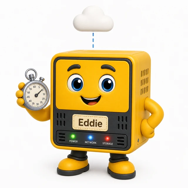
Edge Eddie
“Send the decision, not the raw feed — the edge earns its keep in milliseconds and megabytes saved.”
Through this chapter, Eddie shadows each placement call: what runs beside the process, what still travels upstream, and the evidence that proves the split.
8.2 Learning Objectives
By the end of this chapter, you will be able to:
- Define edge, fog, and cloud as workload placement options, not as competing product labels.
- Explain when latency, bandwidth, privacy, reliability, operations, and evidence boundaries push work toward each tier.
- Write a placement decision record that separates telemetry, command, management, and health paths.
- Review an IoT placement claim for degraded-mode behavior, ownership, and retest triggers.
A tier label is not proof. Placement is reviewable only when each workload has a named requirement, measured or testable evidence, a normal path, a degraded path, and an owner.
8.3 The Three-Tier Model
Start by naming the work. A warehouse dock sensor can filter noisy events at the edge, let a fog gateway coordinate local alerts and screens, and send curated history to the cloud for fleet analysis. The tiers are not a ranking. They divide work by timing, scope, evidence, and who can recover the path when a link or service fails.
![]() Eddie’s Edge Ledger
Eddie’s Edge Ledger
- Decide here: the dock sensor filters its own noisy events — first response stays local.
- Send up: curated history for fleet analysis; the fog gateway coordinates local alerts en route.
- Clock it: no number yet — timing and scope divide the work; the drivers table sets the measured bar.

8.3.1 Edge
Handles work that must stay near the device: immediate sensing, local filtering, simple inference, safety interlocks, offline behavior, and first response.
8.3.2 Fog
Handles nearby coordination: gateway decisions, site dashboards, protocol bridging, aggregation, buffering, local policy, and degraded-mode service.
8.3.3 Cloud
Handles broad services: long-term storage, fleet analytics, model training, cross-site reporting, identity governance, update orchestration, and audit records.

8.4 Placement Drivers
Review placement by evidence, not by preference. Write the same workload three ways before choosing a tier: at the edge, what must keep working if the network disappears; at the fog tier, what a site or gateway can coordinate better than a single device; in the cloud, what needs fleet history, model training, governance, or cross-site comparison.
| Driver | Often pushes toward | Evidence to collect | Common mistake |
|---|---|---|---|
| Response time | Edge for immediate control; fog for site response; cloud when delayed response is acceptable. | Measured path latency, jitter, local queueing, actuation time, and degraded-mode behavior. | Using average latency when the decision depends on worst-case or tail behavior. |
| Data volume | Edge or fog when raw streams are too large; cloud when curated history is needed. | Raw rate, filtered rate, retention need, compression rule, link capacity, and exception handling. | Sending every raw sample upstream without proving the cost or value of that transfer. |
| Privacy and control | Edge or fog when sensitive data or physical authority should remain local; cloud for governed fleet services. | Data classification, authorization boundary, audit path, command approval, and local fallback rule. | Mixing telemetry and commands so a dashboard path becomes an uncontrolled control path. |
| Operations | The tier with clear owners, monitoring, update path, rollback, and support access. | Runbooks, health checks, version records, alert ownership, backup, and retest cadence. | Choosing a tier that works in a demo but cannot be patched, observed, or recovered safely. |
![]() Eddie’s Edge Ledger
Eddie’s Edge Ledger
- Decide here: immediate control at the edge when response time drives it.
- Send up: the filtered rate, not every raw sample — unproven raw upload is the table’s named mistake.
- Clock it: measured path latency, jitter, worst-case tail — averages are the wrong evidence.
8.5 Write a Placement Decision Record
A practical edge-fog-cloud review starts by listing workloads, not technologies. Telemetry upload, alarm decision, actuator command, local dashboard, identity check, update delivery, model inference, model training, and audit retention can each have different placement needs. Treat them as separate decisions until the evidence says they can be combined.
For each workload, record:
- Workload: The exact behavior, such as filter readings, raise an alarm, aggregate a site summary, run inference, train a model, store history, or update devices.
- Requirement: Response time, data volume, privacy, safety, reliability, compute, power, connectivity, and support constraints in plain language.
- Chosen tier: The simplest placement that can meet the requirement and can still be operated, monitored, updated, and recovered.
- Paths: Separate telemetry, command, management, identity, update, audit, and health paths instead of drawing one generic arrow.
- Proof: The test, measurement, pilot, operator runbook, and retest trigger that keep the claim bounded.
8.6 Paths and Boundaries
An edge-fog-cloud system is a set of paths that cross trust, timing, and ownership boundaries. A telemetry path may move sensor facts upward. A command path may move decisions downward. A management path may deliver policies, credentials, updates, and rollback controls. A health path may report stale data, missing data, and degraded operation. Each path has a different failure mode.

| Path | What it proves | What it does not prove | Retest trigger |
|---|---|---|---|
| Telemetry upward | Readings, events, summaries, or features can move from device or fog tier toward storage and analytics. | Command safety, local autonomy, dashboard freshness, or field usefulness of every retained value. | Sensor, sampling, filter, aggregation, schema, link, retention, or dashboard change. |
| Command downward | Approved decisions can reach a device or site controller through the reviewed authorization and audit path. | That commands are always safe, timely, reversible, or allowed under degraded connectivity. | Actuator, policy, role, dashboard, authorization, audit, timeout, or fallback change. |
| Management downward | Credentials, configuration, firmware, model artifacts, and policy updates can be delivered and rolled back. | Telemetry quality, business value, or correctness of the workload placement decision. | Certificate, key, update, model, policy, rollback, owner, or support tool change. |
| Health and recovery upward | The system can report offline devices, stale data, buffer state, degraded mode, and recovery status. | That every local decision remained correct during the outage or that no data was lost. | Outage scenario, queue rule, clock behavior, stale-data display, reconciliation, or incident process change. |
8.7 Summary
- Edge, fog, and cloud are placement options for specific workloads, not proof by themselves.
- A reviewable placement claim names the workload, tier, requirement, normal path, degraded path, owner, evidence, and retest trigger.
- Edge often fits immediate local work; fog often fits nearby coordination; cloud often fits fleet services, history, governance, and broad analytics.
- Telemetry, command, management, and health paths need separate evidence because they fail in different ways.
- Strong placement records keep physical authority, privacy, latency, bandwidth, recovery, updates, and monitoring visible before rollout.
Approve edge, fog, and cloud placement only when each workload is tied to its required behavior, evidence boundary, operating owner, degraded-mode rule, and retest trigger.
8.8 See Also
8.8.1 Edge, Fog, and Cloud: Architecture
Map device, gateway, site, regional, and cloud layers with placement evidence and failure boundaries.
8.8.2 Edge-Fog Decision Framework
Use response, data, trust, connectivity, and operations constraints to decide where workloads belong.
8.8.3 Edge-Fog Latency
Build measured response budgets before choosing where control, inference, and dashboards should run.
8.8.4 Edge Bandwidth Optimization
Review filtering, aggregation, compression, batching, and local inference as bandwidth-placement tools.