22 Indoor Positioning: Wi-Fi, UWB, and Sensor Fusion
More
Depth: Practitioner
Progress saves as you read. Mark sections complete as you go; your progress appears in the sidebar.
22.1 Start With the Situation
This section: Start With the Situation — A Bluetooth Low Energy (BLE) deployment can estimate position.
A Bluetooth Low Energy (BLE) deployment can estimate position. Yet multipath, or signals bouncing from walls, and layout changes may make the result too uncertain. A fingerprint is a stored signal pattern for a place. Time of flight measures how long a signal travels; fused motion combines that evidence with movement readings. Compare these methods to decide what accuracy the site can support.
22.2 Overview
This section: Overview — This route compares Wi-Fi, UWB, ultrasonic, and fused sensing, then tests accuracy, calibration, interference, and cost trade-offs.
This route compares Wi-Fi, UWB, ultrasonic, and fused sensing, then tests accuracy, calibration, interference, and cost trade-offs.
This is part 2 of 2. Review Indoor Positioning: BLE Beacons and Ranging when you need the first route.
22.3 Learning Objectives
This section: Learning Objectives
By the end of this chapter, you will be able to:
- design and maintain a Wi-Fi fingerprint map
- explain UWB time-of-flight accuracy and deployment limits
- combine radio and motion evidence for indoor-outdoor transitions
22.4 Wi-Fi Fingerprinting
This section: Wi-Fi Fingerprinting — Wi-Fi fingerprinting maps RSSI patterns to physical locations by pre-surveying the space.
Wi-Fi fingerprinting maps RSSI patterns to physical locations by pre-surveying the space.
Use Figure 22.1 to compare the survey record with a live RSSI pattern before assigning an indoor location.
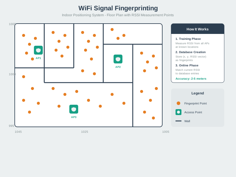
Begin with the offline survey, where several access-point RSSI values are recorded at known reference locations. Walls and other features shape those patterns, so AP3’s weak value may be as informative as AP1’s strong value. During the online phase, the device measures a new vector and compares it with the stored fingerprints. The closest match supplies an estimate, not a direct range. Moved access points, changed furniture, crowds, device calibration, or stale surveys can shift the pattern, so confidence and a survey-maintenance rule belong with the result.
22.4.1 Two-Phase Process
Offline Phase (Survey):
Walk through the space with a device. At each known location, record RSSI from all visible access points. Build a fingerprint database mapping RSSI vectors to locations.
Online Phase (Positioning):
Device scans visible APs and measures RSSI. Compare current RSSI vector to database entries. Find closest match(es) to estimate position.
22.4.2 Challenges with Fingerprinting
Environmental changes: Moved furniture, added walls, relocated APs. Temporal variations: Different occupancy (empty vs. crowded) affects propagation. Device variations: Different phones have different RSSI calibration. Maintenance burden: Plan a site-specific Wi-Fi fingerprint resurvey cadence; 3–6 months can be an initial maintenance assumption.
Mitigation strategies:
Crowd-sourced calibration (users’ movements gradually update database). Hybrid approaches (combine fingerprinting with dead reckoning). Machine learning (automatically detect and adapt to environmental changes).
Fingerprinting reuses infrastructure, while UWB changes the infrastructure to measure time more directly. That trade moves the discussion from survey maintenance to precision ranging.
22.5 Ultra-Wideband (UWB) Positioning
This section: Ultra-Wideband (UWB) Positioning — UWB uses extremely short pulses (nanoseconds) across a wide frequency spectrum (3.1-10.6 GHz), enabling precise time-of-flight measurements.
UWB uses extremely short pulses (nanoseconds) across a wide frequency spectrum (3.1-10.6 GHz), enabling precise time-of-flight measurements.
Key advantages:
10-30cm accuracy: Far exceeds BLE/Wi-Fi. Multipath resistant: Short pulses separate direct and reflected paths. Low interference: Spread spectrum doesn’t interfere with other systems.
Applications:
Hospital equipment tracking (room-level precision). Apple AirTags (precise “find my” direction finding). Autonomous robot navigation. Augmented reality anchoring.
UWB achieves 10-30 cm accuracy through precise time-of-flight measurement. How does the two-way ranging protocol work?
Traditional one-way ToF problem: If transmitter and receiver clocks are not synchronized, measuring gives nonsense (clocks may differ by milliseconds).
Two-way ToF solution:
Tag → Anchor: Tag sends pulse at (tag clock). Anchor processes: Waits known delay (e.g., 500 µs). Anchor → Tag: Anchor replies at (anchor clock). Tag measures round-trip: (tag clock only). Anchor reports: “I replied after from receiving”.
Distance calculation:
Example with numbers:
Tag sends pulse at . Signal travels to anchor (distance m): arrives at ns. Anchor waits µs, then replies. Reply travels back: another 16.67 ns. Tag receives at µs. Measured round-trip: µs.
UWB timing precision: With 500 MHz bandwidth, timing precision ns. This translates to distance precision:
Why real-world accuracy is 10-30 cm (not 30 cm worst-case): Averaging multiple measurements and trilateration from 3+ anchors reduces error by where number of measurements.
The timing calculation becomes a position only when several measured distances meet in a known geometry. The room-plan diagram in Figure 22.2 turns that requirement into an arrangement that exposes both the useful evidence and its dependencies.
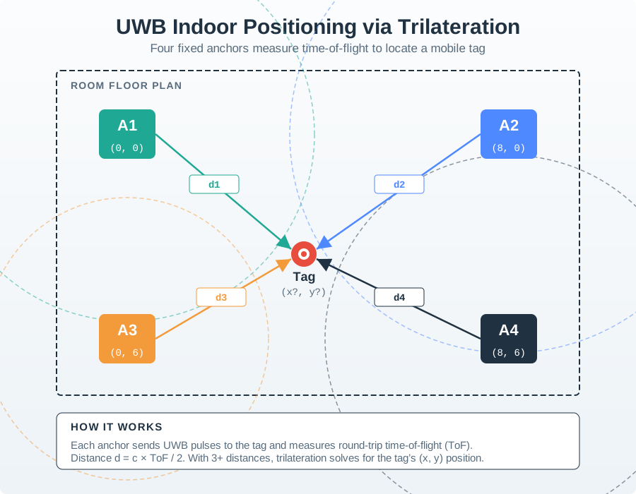
The ROOM FLOOR PLAN diagram in Figure 22.2 fixes anchors A1 (0, 0), A2 (8, 0), A3 (0, 6), and A4 (8, 6) around the unknown Tag (x?, y?). Each link contributes a distance—d1 through d4—from round-trip time of flight. Three distances can solve the two-dimensional position; the fourth adds redundancy for checking noise and obstructed paths. The geometry therefore connects UWB’s pulse timing to the commissioning requirement for surveyed anchors and enough usable lines of sight.
 Checkpoint: Precision Systems
You now know:
- UWB uses short pulses and time-of-flight evidence to reach the chapter’s 10-30 cm accuracy class.
- The gain is strongest for hospital equipment tracking, autonomous robots, augmented reality anchoring, and other high-consequence indoor fixes.
- Precision still depends on anchors, geometry, line-of-sight handling, and site commissioning.
22.6 Sensor Fusion for Seamless Positioning
This section: Sensor Fusion for Seamless Positioning — Real-world applications often require positioning that works both indoors and outdoors.
Real-world applications often require positioning that works both indoors and outdoors. Sensor fusion combines multiple positioning technologies to provide seamless coverage.
Scenario: A delivery driver app must track location seamlessly as the driver moves from outdoor parking (GPS) to indoor warehouse (Wi-Fi/BLE) for package pickup.
Given:
Outdoor GPS position: (37.7749 N, -122.4194 W) with HDOP = 1.2, accuracy = 4.8 meters. GPS signal lost upon entering building (< 4 satellites visible). Indoor Wi-Fi fingerprint match: Warehouse Zone B, confidence 78%. BLE beacon proximity: Beacon “Dock-3” at -62 dBm (estimated 1.5m distance). IMU dead reckoning: 12.3 meters walked at heading 045 since GPS loss. Building floor plan constraint: Driver must be in accessible walkway.
Steps:
Detect GPS degradation:. Satellite count drops from 8 to 3 over 5 seconds. HDOP increases from 1.2 to 6.5 (poor geometry). Trigger: Switch to indoor positioning mode when satellites < 4 AND HDOP > 4.
Initialize indoor position from last GPS fix:. Last valid GPS: (37.7749, -122.4194) at building entrance. Transform to local coordinates: (0, 0) meters at entrance door.
Fuse dead reckoning with Wi-Fi fingerprint:. IMU estimate: (8.7, 8.7) meters from entrance (12.3m at 45 degrees). Wi-Fi fingerprint center: (10.0, 12.0) meters (Zone B centroid). Weighted position estimate: (9.22, 10.02) meters. Weights shown for this calculation: IMU 0.6, Wi-Fi 0.4.
Refine with BLE proximity:. Beacon Dock-3 located at (8.5, 10.0) meters. Proximity constraint: Driver within 1.5m of Dock-3. The BLE proximity observation narrows the possible positions to within 1.5 m of the beacon.
Apply map constraints:. Compare the estimated region with the floor plan. Reject estimates inside walls or shelves and retain only positions in valid walkways.
Result: The fused sensors and map constraint can support a Loading Dock 3 assignment; validate position error against calibrated site measurements before reporting an accuracy value.
Key Insight: Sensor fusion combines sources with different strengths and limitations. GPS provides absolute position outdoors but fails indoors. IMU provides relative movement but drifts over time; Wi-Fi fingerprinting gives zone-level position but requires a pre-surveyed database; BLE beacons provide proximity constraints. Validate the fused estimate with calibrated site measurements before assigning an accuracy value.
No source in the delivery-driver example remains trustworthy across the whole journey. Figure 22.3 shows how complementary measurements enter one estimate while their accuracy and drift determine how much influence each receives.
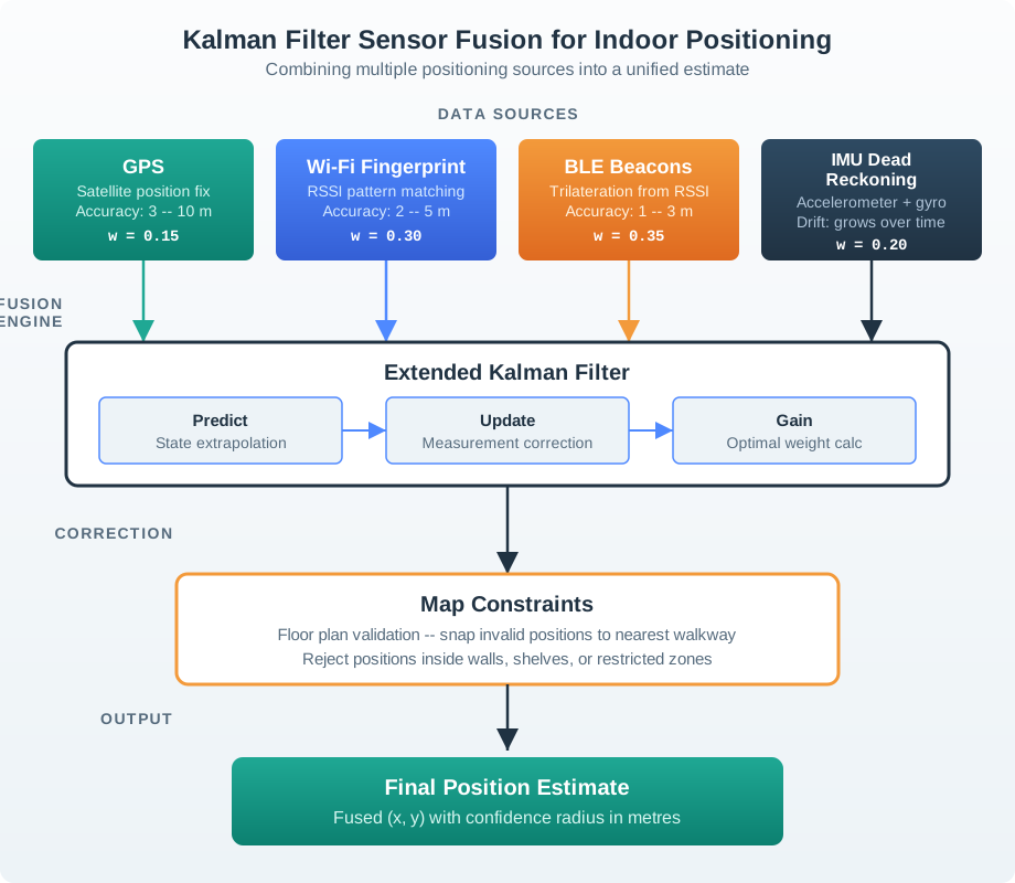
On the data sources side of Figure 22.3, GPS gives a point with an error band of 3–10 m; that band is 10 m - 3 m = 7 m wide. A Wi-Fi site map gives 2–5 m, while BLE gives 1–3 m. The IMU fills motion between fixes, but its drift grows with time. The filter moves between a guess and a new measure. Map rules then reject points inside walls or shelves. The final point keeps a trust radius, so the screen shows doubt from the source instead of hiding it.
The worked examples have named the evidence sources. The next step is turning those measurements into a repeatable implementation path.
22.7 BLE Beacon Trilateration Engine
This section: BLE Beacon Trilateration Engine — This Python implementation computes indoor position from BLE beacon RSSI measurements using the trilateration method from the worked example above.
This Python implementation computes indoor position from BLE beacon RSSI measurements using the trilateration method from the worked example above. It applies RSSI-to-distance conversion, least-squares trilateration, and RSSI averaging to smooth noisy readings:
import math

class BLETrilateration:
    """Estimate indoor position from BLE beacon RSSI measurements.

    Uses the log-distance path loss model to convert RSSI to distance,
    then solves the trilateration system via least-squares.
    """
    def __init__(self, tx_power=-59, path_loss_exp=2.5):
        self.tx_power = tx_power      # RSSI at 1 meter (dBm)
        self.n = path_loss_exp         # Indoor path loss exponent
        self.beacons = {}              # {id: (x, y)}
        self.rssi_history = {}         # {id: [recent RSSI values]}
        self.history_size = 5          # Average last N readings

    def add_beacon(self, beacon_id, x, y):
        """Register a beacon at known coordinates (meters)."""
        self.beacons[beacon_id] = (x, y)
        self.rssi_history[beacon_id] = []

    def rssi_to_distance(self, rssi):
        """Convert RSSI (dBm) to estimated distance (meters)."""
        if rssi >= self.tx_power:
            return 0.1  # Very close
        return 10 ** ((self.tx_power - rssi) / (10 * self.n))

    def update_rssi(self, beacon_id, rssi):
        """Record an RSSI measurement, maintaining rolling average."""
        if beacon_id in self.rssi_history:
            history = self.rssi_history[beacon_id]
            history.append(rssi)
            if len(history) > self.history_size:
                history.pop(0)

    def _averaged_rssi(self, beacon_id):
        """Return smoothed RSSI from recent measurements."""
        history = self.rssi_history.get(beacon_id, [])
        if not history:
            return None
        return sum(history) / len(history)

    def estimate_position(self):
        """Compute position via least-squares trilateration.

        Requires at least 3 beacons with recent RSSI data.
        Returns (x, y, mean_absolute_range_residual_m) or None if insufficient data.
        """
        measurements = []
        for bid, (bx, by) in self.beacons.items():
            avg_rssi = self._averaged_rssi(bid)
            if avg_rssi is not None:
                dist = self.rssi_to_distance(avg_rssi)
                measurements.append((bx, by, dist))

        if len(measurements) < 3:
            return None

        # Least-squares: linearize by subtracting last equation
        # from all others: 2(xi-xn)x + 2(yi-yn)y = dn^2 - di^2 + xi^2 - xn^2 + yi^2 - yn^2
        ref = measurements[-1]
        A_rows, b_rows = [], []
        for bx, by, d in measurements[:-1]:
            A_rows.append([2 * (bx - ref[0]), 2 * (by - ref[1])])
            b_rows.append(ref[2]**2 - d**2 + bx**2 - ref[0]**2 + by**2 - ref[1]**2)

        # Solve via pseudo-inverse (A^T A)^-1 A^T b
        # Manual 2x2 for simplicity
        a11 = sum(r[0]**2 for r in A_rows)
        a12 = sum(r[0] * r[1] for r in A_rows)
        a22 = sum(r[1]**2 for r in A_rows)
        b1 = sum(A_rows[i][0] * b_rows[i] for i in range(len(b_rows)))
        b2 = sum(A_rows[i][1] * b_rows[i] for i in range(len(b_rows)))

        det = a11 * a22 - a12 * a12
        if abs(det) < 1e-10:
            return None

        x = (a22 * b1 - a12 * b2) / det
        y = (a11 * b2 - a12 * b1) / det

        # Compute mean absolute range residual; this is not position accuracy
        residuals = []
        for bx, by, d in measurements:
            est_d = math.sqrt((x - bx)**2 + (y - by)**2)
            residuals.append(abs(est_d - d))
        mean_range_residual = sum(residuals) / len(residuals)

        return round(x, 2), round(y, 2), round(mean_range_residual, 2)

# Example: Museum indoor wayfinding
tri = BLETrilateration(tx_power=-59, path_loss_exp=2.5)
tri.add_beacon("entrance", 0, 0)
tri.add_beacon("gift-shop", 10, 0)
tri.add_beacon("cafe", 5, 8)

# Simulate visitor walking near entrance
for rssi in [-64, -65, -66, -65, -64]:  # 5 readings from entrance beacon
    tri.update_rssi("entrance", rssi)
for rssi in [-82.3, -82.3, -82.3, -82.3, -82.3]:  # gift-shop beacon
    tri.update_rssi("gift-shop", rssi)
for rssi in [-81.6, -81.6, -81.6, -81.6, -81.6]:  # cafe beacon
    tri.update_rssi("cafe", rssi)

result = tri.estimate_position()
if result:
    x, y, residual = result
    print(f"Estimated position: ({x}, {y}) meters")
    print(f"Mean absolute range residual: {residual} meters")

# Show RSSI-to-distance conversion
for bid in tri.beacons:
    avg = tri._averaged_rssi(bid)
    dist = tri.rssi_to_distance(avg)
    print(f"  {bid}: RSSI={avg:.0f} dBm -> {dist:.2f}m")
# Output:
# Estimated position: (1.49, 0.80) meters
# Mean absolute range residual: 0.01 meters
#   entrance: RSSI=-65 dBm -> 1.74m
#   gift-shop: RSSI=-82 dBm -> 8.55m
#   cafe: RSSI=-82 dBm -> 8.02m
The reported mean absolute range residual summarizes the fitted ranges; it is not coordinate error or a confidence bound. Quantify position error with calibrated site measurements. The path_loss_exp parameter must be calibrated on-site because it changes the estimated ranges and position.
Checkpoint: Fusion and Implementation
You now know:
- Sensor fusion weights GPS, Wi-Fi, BLE, IMU, and map constraints by reliability rather than trusting a single source everywhere.
- A Kalman filter can smooth the indoor-outdoor handoff, but the UI still needs freshness, confidence, and source-quality signals.
- The BLE engine is only as good as its calibrated path loss exponent, RSSI averaging, beacon geometry, and map constraints.
22.8 Knowledge Check
This section: Knowledge Check
Scenario: A 500-bed hospital needs real-time location tracking for 2,000 medical devices (wheelchairs, IV pumps, portable monitors) to reduce search time and improve utilization.
Requirements:
Room-level accuracy (identify which room equipment is in). 3-second update rate when device moves. 10-year battery life for portable equipment. $50,000 budget for infrastructure deployment. Works across 5 floors with concrete walls and metal equipment.
Technology Comparison:
| Technology | Accuracy | Battery Life | Infrastructure Cost | Total Cost | Suitable? |
|---|---|---|---|---|---|
| UWB | 10-30 cm | 2-3 years | $80,000 (200 anchors × $400) | $280,000 | Too expensive |
| Wi-Fi RSSI | 3-5 m | 1 year (frequent scanning) | $0 (existing APs) | $50,000 | Poor battery life |
| BLE Beacons | 1-3 m | 5-7 years | $15,000 (500 beacons × $30) | $65,000 | Best fit, pending battery redesign |
Decision: The listed BLE design fits the $50,000 infrastructure cap, but its stated 5–7-year battery life misses the 10-year requirement. Validate a different tag/power plan or revise that requirement before deployment.
Implementation Details:
Beacon Placement: Mount beacons on ceiling every 10 meters in grid pattern. RSSI Calibration: Survey 50 sample locations, measure RSSI at 1m, 3m, 5m distances. Path Loss Exponent: Concrete hospital = n=3.2 (higher than open space n=2.0). Trilateration: Each asset tag hears 4-6 beacons, computes position via least-squares. Map Constraints: Positions snapped to valid corridors/rooms, not inside walls. Update Rate: Tags scan every 3 seconds when moving (accelerometer-triggered), every 60 seconds when stationary.
Expected Performance:
Room-level assignment performance: validate with calibrated site measurements before deployment. Battery Life: 6 years for CR2032 coin cell (3 sec updates when moving). Deployment Time: 2 weeks (beacon installation + RSSI survey). Search Time Reduction: From 8 minutes average to 30 seconds.
Key Insight: UWB provides finer positioning than BLE but has a higher infrastructure cost and shorter listed battery life. For hospital asset tracking, room-level accuracy may be sufficient; validate room assignment performance and the tag power plan against the deployment requirements.
Use this table to choose the right indoor positioning technology based on your application requirements:
| Decision Factor | BLE Beacons | Wi-Fi Fingerprinting | UWB | Recommendation |
|---|---|---|---|---|
| Accuracy Needed | 1-3m | 3-5m | 10-30cm | Retail/hospitals: BLE; Robotics/AR: UWB |
| Infrastructure Budget | $10k-$50k | $0 (existing) | $50k-$200k | Budget <$50k: BLE or Wi-Fi |
| Deployment Timeline | 2-4 weeks | 4-8 weeks (survey) | 4-6 weeks | Fast: BLE; Existing Wi-Fi: Wi-Fi |
| Battery Life Priority | Compare BLE, Wi-Fi, and UWB with device-specific tag, reporting interval, and battery capacity; avoid generic lifetime bands | |||
| Multipath Resistance | Low (RSSI affected) | Low (RSSI patterns) | High (ToF) | Metal/concrete: UWB |
| Maintenance Effort | Low (replace batteries) | High (re-survey) | Medium | Low maintenance: BLE |
| Scalability | High (1000s of tags) | Medium (database size) | High | Large scale: BLE or UWB |
Decision Tree:
Do you need sub-50cm accuracy? → YES: Compare UWB with site-validated BLE direction finding; NO: Continue. Do you have existing Wi-Fi infrastructure? → YES: Try Wi-Fi fingerprinting | NO: Continue. Is budget <$50k for 50,000 sq ft? → YES: BLE beacons | NO: UWB for best accuracy. Is environment highly metallic/reflective? → YES: UWB (multipath resistant) | NO: BLE sufficient. Do you need 10+ year battery life? → YES: None of the listed tag plans qualifies; validate a different power design. NO: Compare BLE and UWB against the remaining requirements.
Example Applications:
Warehouse asset tracking (10,000 pallets): BLE beacons (low cost, zone-level accuracy sufficient). Museum visitor navigation (5,000 visitors/day): Wi-Fi fingerprinting (leverage existing network, no tags needed). Factory robot navigation (20 AGVs): UWB (centimeter precision required, small number of tags). Hospital equipment tracking (2,000 devices): BLE beacons (room-level accuracy, long battery life). Retail customer analytics (500 shoppers): BLE beacons (opt-in via app, privacy-preserving).
The Mistake: Deploying BLE beacons with default path loss parameters (TxPower = -59 dBm, n = 2.0) without on-site calibration, assuming datasheet values work in all environments.
Why It Fails:
The path loss exponent n varies dramatically by environment:
| Environment | Typical n | Impact on Distance Error |
|---|---|---|
| Free space (outdoor) | 2.0 | Baseline (datasheet) |
| Office (drywall) | 2.5 | Depends on RSSI and reference-distance calibration |
| Hospital (concrete) | 3.2 | Depends on RSSI and reference-distance calibration |
| Factory (metal) | 3.8 | Depends on RSSI and reference-distance calibration |
Illustrative deployment failure: A hypothetical retail example shows an 8 m estimate for a beacon actually 3 m away when the path-loss model is uncalibrated; use measured RSSI and reference distances for any deployment claim.
The Cost: A wrong path-loss exponent can produce large site-dependent range and position errors. Measure RSSI at known distances and test zone decisions before deployment; an exponent pair alone does not determine a unique position error.
How to Fix It:
- Conduct RSSI survey: Place beacon at known location, measure RSSI at 1m, 3m, 5m, 10m distances
- Calculate actual n: Use formula n = (RSSI₁ - RSSI₂) / (10 × log₁₀(d₂/d₁))
- Test in 10 locations: Verify calibrated n works across entire deployment area
- Document per-zone: Large buildings may need different n for different zones (concrete basement vs. glass atrium)
Calibration Example:
Given measurements:
- RSSI at 1m = -59 dBm
- RSSI at 5m = -75 dBm
Calculate n: n = (-59 - (-75)) / (10 × log₁₀(5/1)) = 16 / (10 × 0.699) = 2.29
Interactive Calibration: Use your own RSSI measurements to calculate the actual path loss exponent for your environment. This calibrated value should replace the default n=2.5 in your deployment.
Time Investment: 4-8 hours of RSSI surveying saves months of troubleshooting positioning errors post-deployment.
Key Insight: Never deploy indoor positioning without calibration. Datasheet values are laboratory measurements in free space—real buildings have walls, metal, people, and furniture that change RF propagation. Calibrate or fail.
Checkpoint: Selection and Calibration
You now know:
- Technology choice is an accuracy, cost, battery, infrastructure, maintenance, and privacy decision.
- BLE can fit large room-level deployments, UWB can justify its cost for tighter precision, and Wi-Fi fingerprinting depends on a living survey.
- Calibration is part of launch: path loss, map constraints, anchor health, and regression routes decide whether the system keeps working after the building changes.
Common Pitfalls
This section: Common Pitfalls
Adding too many features before validating core user needs wastes weeks of effort on a direction that user testing reveals is wrong. IoT projects frequently discover that users want simpler interactions than engineers assumed. Define and test a minimum viable version first, then add complexity only in response to validated user requirements.
Treating security as a phase-2 concern results in architectures (hardcoded credentials, unencrypted channels, no firmware signing) that are expensive to remediate after deployment. Include security requirements in the initial design review, even for prototypes, because prototype patterns become production patterns.
Designing only for the happy path leaves a system that cannot recover gracefully from sensor failures, connectivity outages, or cloud unavailability. Explicitly design and test the behaviour for each failure mode and ensure devices fall back to a safe, locally functional state during outages.
22.9 Summary
This section: Summary — BLE Beacons: Low cost, 1-3m accuracy, requires beacon deployment.
Indoor Positioning Technologies:
BLE Beacons: Low cost, 1-3m accuracy, requires beacon deployment. Wi-Fi Fingerprinting: Uses existing infrastructure, 3-5m accuracy, labor-intensive survey. UWB: High precision (10-30cm), multipath resistant, higher cost. Ultrasonic: Best accuracy (3cm) but expensive and requires line-of-sight.
Key Trade-offs:
Accuracy vs. Cost: UWB is most accurate but most expensive. Infrastructure vs. Opportunistic: Wi-Fi reuses existing APs, BLE/UWB require deployment. Power vs. Update Rate: Frequent positioning updates drain batteries.
Sensor Fusion Principles:
Combine multiple technologies for seamless indoor-outdoor coverage. Weight sources by reliability (GPS high outdoors, low indoors). Use Kalman filters to smooth transitions and handle sensor failures. Apply map constraints to prevent impossible positions (inside walls).
Indoor positioning requires fundamentally different technologies from outdoor GPS because satellite signals cannot penetrate buildings. The choice between BLE beacons (cheap, 1-3m), Wi-Fi (free infrastructure, 3-5m), and UWB (expensive, 10-30cm) depends on accuracy requirements, budget, and existing infrastructure. The most robust real-world systems use sensor fusion, combining multiple technologies through Kalman filters to smooth transitions and handle individual sensor failures. The key insight: no single positioning technology works everywhere — seamless location awareness requires intelligent fusion of multiple sources.
Indoor positioning is like finding your way in a building without any windows to see the sky!
22.9.1 Indoor Treasure Hunt
The Sensor Squad was running a treasure hunt inside a huge shopping mall. But there was a problem — GPS didn’t work indoors!
“My GPS says I’m OUTSIDE!” cried the LED, standing right in the middle of the food court. “The satellite signals can’t get through the roof!”
“Don’t worry!” said Temperature Terry. “We have INDOOR tools!”
Tool 1: Bluetooth Beacons (The Lighthouse Method) the microcontroller placed tiny Bluetooth beacons around the mall. Each one continuously shouted: “I’m at the food court!” or “I’m at the shoe store!” When Lila’s phone heard a beacon, it knew she was nearby.
“But how CLOSE am I?” asked Lila. “The beacon’s signal gets WEAKER the farther you walk. If I measure the signal strength from THREE beacons, I can figure out exactly where I am — just like GPS uses three satellites!” said Sammy.
Tool 2: Wi-Fi Fingerprinting (The Memory Method) the battery had walked through every corridor last week, recording what Wi-Fi signals looked like at each spot. “At the pet store, I can see Wi-Fi networks ‘MallGuest’ at -60, ‘StoreWifi’ at -45, and ‘CoffeeShop’ at -72. This PATTERN is unique to the pet store!”
Now when someone’s phone sees that same Wi-Fi pattern, the system says “You must be near the pet store!” It’s like recognizing a song by its melody!
Tool 3: UWB (The Stopwatch Method) For the FINAL treasure (hidden on a specific shelf), they needed ultra-precise tracking. UWB sent super-quick pulses and measured the EXACT time they took to bounce back. “10 centimeters accuracy!” cheered Max. “I can tell which SHELF the treasure is on!”
The Grand Fusion “The best part,” said Sammy, “is we can use ALL of these together! Wi-Fi gives us the general area, Bluetooth narrows it to the right store, and UWB pinpoints the exact spot. It’s like using a map, then a compass, then a magnifying glass!”
22.9.2 Key Words for Kids
| Word | What It Means |
|---|---|
| BLE Beacon | A tiny device that broadcasts “I’m here!” using Bluetooth — like a small indoor lighthouse |
| Wi-Fi Fingerprint | The unique pattern of Wi-Fi signals at each location, like a musical chord that’s different everywhere |
| UWB | Ultra-Wideband — sends super-fast pulses to measure distance within centimeters |
| Sensor Fusion | Combining multiple tools together for the best answer (like asking three friends instead of one) |
How this chapter connects to other IoT concepts:
Compensates for: GPS Limitations which fail indoors due to signal attenuation through building materials. Uses: BLE Beacon Positioning for proximity detection from repeated beacon broadcasts and RSSI measurements. Alternative: UWB Positioning for centimeter-level accuracy via time-of-flight ranging. Fusion with: Sensor Fusion where IMU accelerometer and gyroscope data bridge GPS outages during indoor transitions. Applied in: Asset Tracking hospitals and warehouses track equipment with BLE or UWB systems.
Related topics for deeper exploration:
RSSI Path Loss Models: Mathematical models for converting signal strength to distance estimates. Kalman Filtering for Sensor Fusion: How to combine GPS, Wi-Fi, BLE, and IMU measurements with state-estimation math. Wi-Fi Fingerprinting Databases: Data structures and algorithms for storing and querying RSSI signatures. UWB Positioning Systems: Detailed coverage of UWB anchor deployment and time-difference-of-arrival calculations. Hospital RTLS Case Studies: Real-world implementations of indoor positioning in medical facilities.
Hands-on exercises to explore indoor positioning:
22.9.3 Exercise 1: BLE Beacon RSSI Calibration
Deploy a BLE beacon and measure RSSI at known distances:
- Place beacon at fixed location
- Measure RSSI at 1m, 2m, 3m, 5m, 10m distances
- Plot RSSI vs. log(distance) graph
- Calculate path loss exponent n using formula: n = (RSSI₁ - RSSI₂) / (10 × log₁₀(d₂/d₁))
- Compare measured n to theoretical values (2.0 free space, 2.5-4.0 indoors)
What to observe: RSSI varies at fixed distance, and path-loss exponent depends on environment. Using an incorrect exponent can substantially bias RSSI distance estimates; quantify the error only for specified RSSI and true exponent.
22.9.4 Exercise 2: Wi-Fi Fingerprinting Survey
Create a simple fingerprint database for one room:
- Choose 5 locations in room (corners + center)
- At each location, record RSSI from 3-5 visible Wi-Fi access points
- Create fingerprint map: {location → [RSSI_AP1, RSSI_AP2, …]}
- Test positioning: Stand at unknown location, scan Wi-Fi, find closest fingerprint match
What to observe: Fingerprint matching provides 2-5m accuracy in static environment. Notice how RSSI changes with body orientation (your body attenuates signals). Test again next day—accuracy degrades if anything moved (furniture, people). This demonstrates maintenance burden of fingerprinting.
22.9.5 Exercise 3: Trilateration Geometry
Manually calculate position from 3 beacon distances:
- Place 3 beacons at known positions: A=(0,0), B=(10,0), C=(5,8) meters
- Measure RSSI from each beacon, convert to distances using path loss formula
- Draw circles with radius = estimated distance around each beacon on graph paper
- Find intersection point—that’s your estimated position
- Compare to actual position
What to observe: Circles rarely intersect at a single point due to RSSI noise—they form a small triangle. In this n=2.5 log-distance example, ±3 dBm changes estimated range by about −24%/+32%; multilateration position error depends on anchor geometry.
22.10 What’s Next
This section: What’s Next — Continue to Location Privacy and Regulations to learn about privacy-preserving design patterns, E911 mandates, and ethical considerations when collecting location data.
Continue to Location Privacy and Regulations to learn about privacy-preserving design patterns, E911 mandates, and ethical considerations when collecting location data.
| Previous | Up | Next |
|---|---|---|
| GPS Accuracy and Enhancement | UX Design | Location Privacy and Regulations |
Find help
3 reviewed answers.
Where should I start in a module?
Open the module page from the sidebar to see its chapters in order. Use the module map to return to a topic you need.
Modules and pathsReviewed
What can I try when a project does not work?
Check the symptom, then work through the diagnostic steps. Keep the error message and the smallest example that reproduces it.
When you are stuckReviewed
How do interactive examples work?
Use the interactive guide to check how examples and simulations work before changing your project.
Interactive examples guideReviewed