3 LPWAN Link Budget and Range
Signal Accounting, Path Loss, Margin, Gateway Density, and Field Validation
LPWAN link budget, allowable path loss, receiver sensitivity, fade margin, path loss, gateway density, coverage validation
3.1 Start Simple
Picture a sensor at the edge of a field and a gateway on a roof. The first question is not whether the brochure says long range. The first question is whether enough signal remains after walls, terrain, antenna choices, and uncertainty have taken their share. A link budget is the plain ledger that shows whether a pilot has margin or whether the design needs another gateway, a better antenna, or a different placement.

Phoebe’s Why
A link budget is signal accounting because every term in it, including receiver sensitivity, is a boundary drawn in decibels. Sensitivity is not a fixed property of the radio chip; it is the noise floor the demodulator needs to beat, and LoRa’s spreading factor changes that boundary on purpose. Each higher spreading factor spreads the same information over more chips, so the receiver integrates energy over a longer symbol before deciding what was sent. Averaging over more chips does not add power, but it does average down the noise relative to the signal – exactly the same “more looks, less noise” trick that makes oversampling improve an ADC reading – so the demodulator can pull a correct decision out of a weaker, noisier signal. That is a sensitivity gain, and in this chapter’s ledger a sensitivity gain adds dB for dB straight onto the allowable path loss.
The Derivation
The raw budget this chapter builds is signal minus loss compared with the receiver floor:
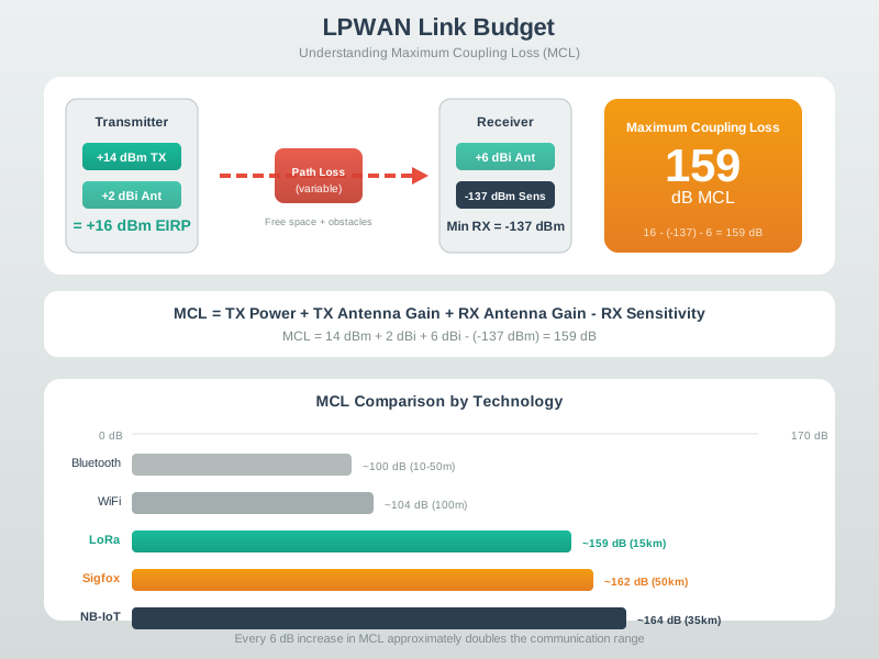
\[\mathrm{Budget} = P_t + G_t + G_r - L - \mathrm{Sensitivity}\]
Allowable path loss is what remains after reserved margin is subtracted:
\[\mathrm{PL}_{allow} = \mathrm{Budget} - \mathrm{Margin}_{reserved}\]
Spreading a symbol over \(2^{SF}\) chips integrates that many independent noise samples, giving a processing gain of:
\[G_{SF}(\text{dB}) = 10\log_{10}(2^{SF}) = 3.01\,SF\ \text{dB}\]
so each additional spreading factor step buys roughly \(3.01\) dB more sensitivity, and hence \(3.01\) dB more allowable path loss.
Worked Numbers: This Chapter’s Own 14 dBm Link
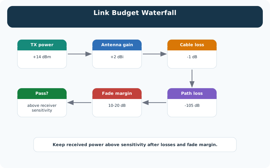
- Raw budget, from the chapter’s own figures (14 dBm TX, 2 dBi device antenna, 6 dBi gateway antenna, 3 dB total loss, \(-130\) dBm sensitivity): \(14+2+6-3-(-130)=149\) dB – exactly the 149 dB raw budget quoted above
- Allowable path loss after the chapter’s own 10+12+4 = 26 dB reserved margin: \(149-26=123\) dB – exactly the 123 dB figure quoted above
- Theoretical SF gain, SF10 to SF12 (2 steps): \(2\times3.01=6.02\) dB
- Catalog-typical SX1276-class sensitivity steps at 125 kHz bandwidth (datasheet-typical, confirm per radio): SF7 \(-123\), SF8 \(-126\), SF9 \(-129\), SF10 \(-132\), SF11 \(-134.5\), SF12 \(-137\) dBm – each step costs almost exactly the theoretical 3.01 dB, with the last two steps landing slightly under it (2.5 dB) from real demodulator implementation loss
- What that buys the ledger: the chapter’s own \(-130\) dBm sensitivity sits between the catalog SF9 and SF10 figures above; moving that same link to a SF12-class \(-137\) dBm floor adds \(137-130=7\) dB of real sensitivity, which would raise the 123 dB allowable path loss to \(123+7=130\) dB – the same reserved-margin ledger, with more spreading-factor room to spend on distance instead of a bigger antenna or another gateway
Overview: Link Budget Is Signal Accounting
An LPWAN link budget is a review record, not a range promise. It adds the useful signal contributions, subtracts losses, compares the expected received signal with receiver sensitivity, and keeps margin for fading, clutter, antenna placement, enclosure loss, and measurement uncertainty.
The result is not "this device reaches ten kilometers." The result is a bounded statement: under these assumptions, this link has enough or not enough remaining margin to justify a pilot.
Suppose a farm water-monitoring project wants one gateway to cover hill tanks, buried meter pits, and a shed-mounted pressure sensor. The radio ledger may begin with a healthy raw budget, but the buried pits need enclosure and ground-level penalties, the shed sensor needs wall-loss allowance, and the hill tanks need wind-driven antenna alignment checks. If the raw budget is 149 dB and the review reserves 10 dB for fading, 12 dB for obstruction, and 4 dB for installation uncertainty, only 123 dB remains for path loss. A model estimate of 118 dB is a pilot candidate; an estimate of 128 dB is not a "maybe" range claim. It is a design gap unless the team changes antenna placement, gateway density, radio settings, or the device location.
The overview record should therefore state the acceptance rule before field work starts. A pass might mean every representative location keeps at least the reserved margin while using an allowed data rate and legal transmit setting. A conditional pass might allow the hill tanks but require a second gateway for buried pits. A fail should name the design change, not leave a vague note that the range was shorter than expected.
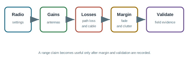
Signal Sources
Transmit power, transmitter antenna gain, receiver antenna gain, radio setting, and receiver sensitivity.
Losses
Cables, connectors, enclosure effects, antenna mismatch, path loss, indoor penetration, foliage, terrain, and clutter.
Margin
Reserved budget for fading, shadowing, seasonal change, installation variation, interference, and measurement uncertainty.
Practitioner: Turn the Ledger into a Margin Decision
Start by calculating raw link budget, then remove the margins and allowances that should not be spent by normal path loss. What remains is maximum allowable path loss. That value can be compared with a model estimate or measured field result.
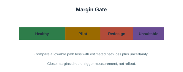
Review habit: state whether the margin result supports rollout, a limited pilot, redesign, or rejection. A link budget without a decision is only arithmetic.
The practitioner decision should also name the evidence owner. If the gateway is moved from a mast to a building wall, the link-budget owner must rerun the allowance, not simply reuse the earlier pass result. If a product team adds confirmed messages or a larger payload, the margin gate should be reopened because retry behavior and airtime can turn a coverage pass into an operations failure. The ledger is strongest when it records both the numeric answer and the condition that would make that answer stale.
Under the Hood: Models Need Field Evidence
Path-loss models translate distance and environment assumptions into estimated loss. A free-space estimate is a clean baseline, while log-distance and clutter-aware models add assumptions about terrain, buildings, foliage, antenna height, and indoor penetration. The model is useful only when its assumptions are documented and tested.
Treat every model output as a hypothesis to challenge. If the model assumes antennas several metres above ground but the real device is bolted inside a metal cabinet, the path-loss estimate is optimistic even when the arithmetic is correct. If the model assumes clear outdoor terrain but the deployment has wet foliage, reinforced concrete, or a service vehicle parked beside the enclosure, the field record must either measure those conditions or reserve enough margin to survive them. Gateway density is the same kind of under-the-hood question. One gateway may satisfy a coverage model yet still create weak receive diversity, high channel load, poor downlink opportunity, or fragile incident response. The release evidence should connect path-loss samples, gateway count, traffic pattern, and retest triggers into one decision.
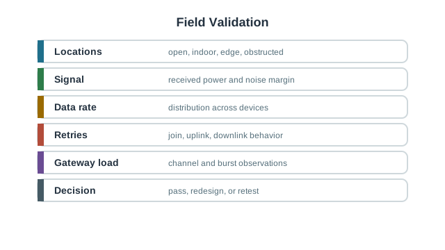
Make the acceptance threshold explicit in the same record. For a rollout gate, the team might require each representative device class to keep reserved margin, join without repeated retries, avoid spending most traffic at the slowest data rate, and show at least one retest trigger for seasonal or installation change. Those criteria keep the model, the measurement, and the release decision tied together.
Coverage
Can each device reach at least one suitable gateway with enough link margin in representative conditions?
Capacity
Can the network absorb joins, retries, confirmed messages, downlinks, bursts, and gateway channel load?
Diversity
Do multiple gateways, better placement, or antenna changes reduce edge-device risk without masking traffic problems?
Validation
Do field tests cover edge, obstructed, indoor, low-antenna, and seasonal cases instead of only easy locations?
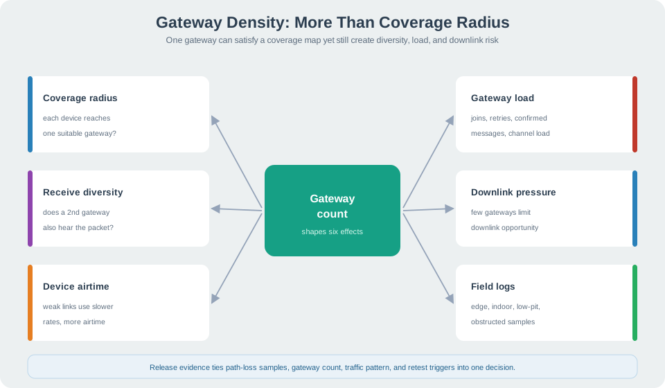
A field team should therefore test the awkward cases on purpose. Put one device in the lowest meter pit, one behind the metal shed wall, one at the edge of the service area, and one near the busiest reporting cluster. Record received signal, noise margin, spreading factor or data-rate distribution, retries, join behavior, gateway identity, and whether a second gateway also heard the packet. If every easy point passes but the low pit consumes all reserved margin, the correct result is not "range proven"; it is "coverage depends on installation constraints." If many edge devices pass only at the slowest rate, the team should also check airtime and downlink pressure before approving the gateway count.
3.2 Summary
- LPWAN link budgets are evidence records, not guaranteed range claims.
- The ledger must show transmit power, antenna gains, implementation losses, receiver sensitivity, path-loss assumptions, and reserved margin.
- Maximum allowable path loss is raw link budget after subtracting fade, clutter, penetration, and uncertainty allowances.
- Coverage planning and capacity planning are separate gates; gateway density must consider both.
- Field validation should test representative difficult locations and define retest triggers for later changes.
3.3 Key Takeaway
A link budget is trustworthy when another engineer can audit the gains, losses, assumptions, margins, model, field samples, and final coverage decision.