6 Point Clouds from Radar and Lidar

6.1 Start With the Story

Radio Remi sees two maps of the same loading area. Lidar draws sharp walls with many points. Radar shows fewer points, but some carry radial speed and radar cross-section. A moving trolley becomes several returns in each frame. Remi must align the sensor pose, remove implausible points, group neighbours, and track a cluster without pretending every dot is an object.

6.2 Overview

A point cloud is a set of detections in a coordinate frame. Lidar points commonly carry 3D position, intensity, and time. Radar detections may carry range, azimuth, Cartesian position, RCS, radial velocity, sensor identity, and time. Vehicle or robot pose places sensor points into a shared frame. Filtering removes only points that fail stated rules; clustering proposes objects; tracking links proposals over time with uncertainty.

6.3 Learning Objectives

By the end of this chapter, you will be able to:

• Read radar and lidar points with position, intensity or RCS, velocity, timestamp, and pose fields.
• Apply coordinate transforms, filtering, clustering, and simple tracking.
• Report missed objects, false clusters, and dataset limits before making an IoT claim.

6.4 Represent every point with context

Coordinates are meaningless without a frame and unit. Sensor-frame points move with the device; world-frame points require a pose transform. Timestamps matter because the platform and targets can move during collection. RCS and intensity are sensor-dependent return measures, not universal material labels. Radial velocity measures motion along the radar line of sight, not full object speed.

6.5 Read the processing chain

The diagram starts with radar and lidar records that keep their different fields. The next card aligns time and pose, then applies bounded range, quality, and motion filters. The final card clusters neighbouring points and associates them over time. Read the uncertainty strip last: every transform, threshold, and association can create missed points, false groups, or identity swaps.

Figure Figure 6.1 keeps the stages in reading order. The diagram starts with radar and lidar records that keep their different fields.

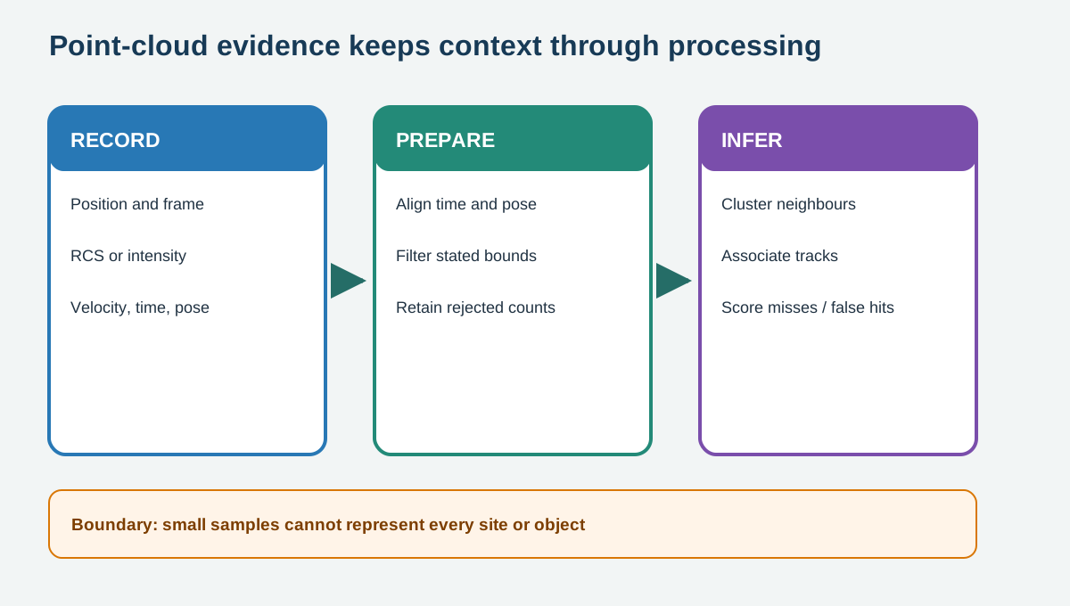
In Figure 6.1, read left to right, then use the final boundary note to limit the conclusion. The arrows show processing order, not proof that the final output is correct in every setting.

6.6 Filter and cluster sparse returns

A range gate removes detections outside the application envelope. Quality or RCS thresholds can suppress noise but may also remove weak people or surfaces. A connected-neighbour cluster joins points within a chosen distance and minimum count. Radar usually needs different thresholds from dense lidar. Tune on training scenes, then preserve a held-out scene so the result is not judged on the same points that set the rules.

6.7 Track and score

A simple tracker predicts a cluster position, finds a compatible new cluster, and updates the track. Gating limits unlikely matches; track age and missed-update counts support deletion. Score point or cluster precision and recall, missed objects, false clusters, and identity switches. A small sample cannot represent all roads, rooms, weather, mounts, or people.

6.8 Dataset and synthetic boundaries

The lab includes a small derived sample from RadarScenes sequence 158. RadarScenes is licensed CC BY-NC-SA 4.0 and supplies automotive radar detections with point-wise labels and track IDs. The lidar room scan is synthetic because no compatible small public scan was selected for this wave. Both files are for teaching the pipeline; neither validates a product or a new environment.

6.9 Decision and Trade-offs

Keep radar when radial velocity and weather tolerance matter, but plan for sparse, ambiguous returns. Keep lidar when dense geometry matters and optical conditions, cleaning, power, and cost fit. Fuse them only after timestamps, coordinate frames, coverage, and failure independence are tested. A merged picture is not automatically more truthful than either input.

6.10 Practice the Method

The linked lab uses a prepared online tool and retains its result evidence. Complete the steps, compare the result with the chapter boundary, and name one condition that the exercise did not test.

6.11 Check Your Reasoning

6.12 Summary

The useful output is an auditable chain from timestamped sensor records to scored associations. Preserve the source frame, filtering rules, clustering settings, track state, and rejected points beside the final objects. That chain shows whether an apparent improvement came from better sensing, a tuned threshold, or a scoring rule that hid difficult cases.

• A point is useful only with its frame, unit, time, sensor, and quality fields.
• Filtering, clustering, and tracking introduce thresholds whose errors must be scored.
• The RadarScenes subset and synthetic lidar scan teach processing, not site or product validation.