Filter, cluster, and track radar and lidar points
Compare an attributed RadarScenes frame with a synthetic lidar room scan, then retain errors and licence boundaries in the result.

Radio Remi: I want you to predict the result, inspect each intermediate value, and keep the final claim inside the evidence.
Predict the reading, then compare it with the measurement.
Python 3 in your browser (JupyterLite)
Python · no installCompare an attributed RadarScenes frame with a synthetic lidar room scan, then retain errors and licence boundaries in the result.
Open the notebook in your browser and run each Python cell; no install or account is needed.
Three ways to run: use JupyterLite here with no install; run main.py locally from the downloadable lab folder; or open the same notebook in Google Colab.
Steps
Step 1
- Do
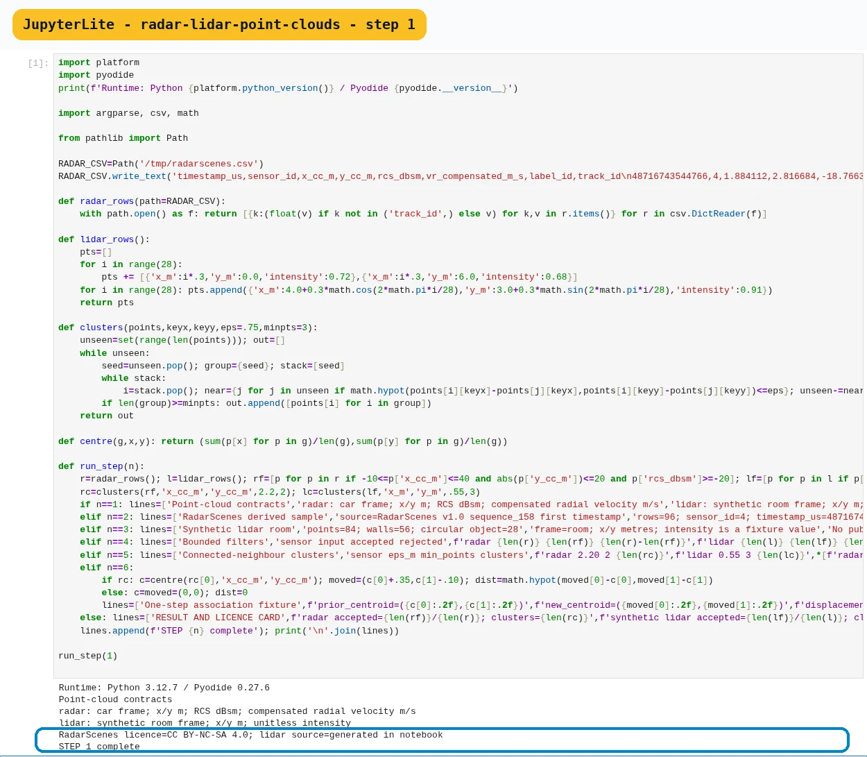
- Inspect the two data contracts.
- You will see
- Radar and lidar columns, coordinate frame, units, licence, and synthetic status are printed.
- Why it matters
- Coordinates are meaningless without a frame and unit.
Step 1 · Python 3 in your browser (JupyterLite); numbered callout added to a real capture. Enlarge screenshot (new tab) Step 2
- Do
- Load the RadarScenes sample.
- You will see
- The notebook reports 96 detections from one timestamp in sequence 158.
- Why it matters
- The lab includes a small derived sample from RadarScenes sequence 158.

Step 2 · Python 3 in your browser (JupyterLite); numbered callout added to a real capture. Enlarge screenshot (new tab) Step 3
- Do
- Generate the synthetic lidar room.
- You will see
- A wall-and-object scan is created with 84 points and an explicit synthetic label.
- Why it matters
- The lidar room scan is synthetic because no compatible small public scan was selected for this wave.

Step 3 · Python 3 in your browser (JupyterLite); numbered callout added to a real capture. Enlarge screenshot (new tab) Step 4
- Do
- Apply bounded filters.
- You will see
- Accepted and rejected point counts appear for each sensor.
- Why it matters
- Filtering removes only points that fail stated rules; clustering proposes objects; tracking links proposals over time with uncertainty.

Step 4 · Python 3 in your browser (JupyterLite); numbered callout added to a real capture. Enlarge screenshot (new tab) Step 5
- Do
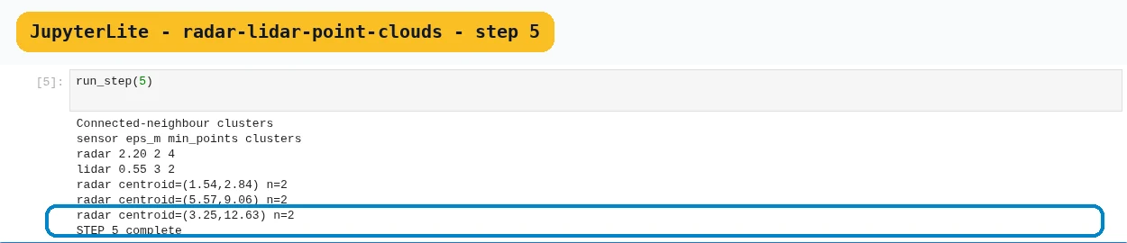
- Cluster connected neighbours.
- You will see
- Cluster counts and centroids are printed with the chosen distance and minimum count.
- Why it matters
- A connected-neighbour cluster joins points within a chosen distance and minimum count.
Step 5 · Python 3 in your browser (JupyterLite); numbered callout added to a real capture. Enlarge screenshot (new tab) Step 6
- Do
- Associate a moved cluster.
- You will see
- The nearest compatible centroid is linked and the displacement is reported.
- Why it matters
- A simple tracker predicts a cluster position, finds a compatible new cluster, and updates the track.

Step 6 · Python 3 in your browser (JupyterLite); numbered callout added to a real capture. Enlarge screenshot (new tab) Step 7
- Do
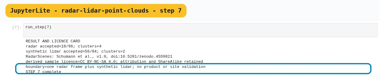
- Write the result and licence card.
- You will see
- The card reports counts, errors, attribution, ShareAlike, and missing validation.
- Why it matters
- Both files are for teaching the pipeline; neither validates a product or a new environment.
Step 7 · Python 3 in your browser (JupyterLite); numbered callout added to a real capture. Enlarge screenshot (new tab)
Chapter checks
These questions refer to the chapter’s examples. Use the return links to review their answers.
What must accompany point coordinates before sensors can be compared?
Return to the chapter’s knowledge checkWhy tune clustering on training scenes and score a held-out scene?
Return to the chapter’s knowledge check