4 FMCW mmWave Radar: Range, Doppler, and Angle

4.1 Start With the Story

Radio Remi is checking a loading bay where dust hides painted floor marks. A camera loses contrast, but a radar return still needs careful reading. Remi sends a rising chirp, mixes the delayed echo with the current transmit signal, and finds a beat tone. Repeating the chirp adds motion evidence. The notebook can recover known simulated targets, but it cannot certify the real bay.

4.2 Overview

Frequency-modulated continuous-wave radar transmits chirps whose frequency changes with time. A delayed reflection returns at a different instantaneous frequency. Mixing transmit and receive signals produces a beat frequency linked to delay and range. Samples within one chirp feed a range FFT; changes across chirps feed a Doppler FFT; phase across antennas supports angle estimation. Resolution and unambiguous limits come from the chosen waveform and sampling system.

4.3 Learning Objectives

By the end of this chapter, you will be able to:

• Relate chirp slope and beat frequency to target range.
• Explain how repeated chirps and antenna phase support Doppler and angle estimates.
• Connect bandwidth, timing, aperture, SNR, resolution, and ambiguity to an IoT claim.

4.4 Chirp, delay, and beat frequency

For a linear chirp, slope equals bandwidth divided by chirp duration. A target at range R creates an approximate round-trip delay of 2R/c. Ignoring target motion for this first step, beat frequency is slope times delay, so range is c times beat frequency divided by twice the slope. The approximation is useful only within the radar’s sampling, calibration, and propagation assumptions.

The mixer removes most of the carrier frequency and leaves a slower beat signal that an analogue-to-digital converter can sample. A larger target or favourable surface may produce a stronger peak, but peak strength is not a direct measure of object size. Leakage between transmitter and receiver can occupy near-range bins and mask a weak reflector. Calibration and windowing shape the spectrum before a range estimator selects candidate peaks.

4.5 Walk through the radar cube

Read the diagram from left to right. The transmit chirp and delayed echo first meet in the mixer. Samples within each chirp form range bins, repeated chirps form Doppler bins, and antenna channels add angle evidence. The output is a detection with range, radial velocity, angle, strength, and uncertainty—not a camera-like object record.

Figure Figure 4.1 keeps the stages in reading order. Read the diagram from left to right.

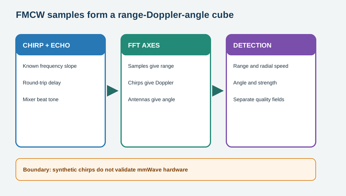
In Figure 4.1, read left to right, then use the final boundary note to limit the conclusion. The arrows show processing order, not proof that the final output is correct in every setting.

4.6 Resolution and ambiguity

Ideal range resolution is approximately c divided by twice the swept bandwidth, so more bandwidth separates closer reflectors. Doppler resolution improves with a longer coherent observation, while frame rate and target change limit how long samples remain comparable. Sampling rate bounds beat frequency and unambiguous range. Pulse timing bounds unambiguous velocity. Windowing reduces spectral leakage but widens peaks.

4.7 Angle and evidence quality

Two receiving antennas observe different phases when a wave reaches them from an angle. An array estimator maps those phase differences to direction under a spacing and calibration model. Grating lobes, multipath, low SNR, mounting error, and a target outside the field of view can make a confident-looking wrong angle. Range, Doppler, and angle should therefore retain separate quality fields before fusion.

4.8 Decision and Trade-offs

Increase bandwidth when close-range separation matters and spectrum, sampling, cost, and regulation permit it. Increase coherent observation time when velocity detail matters and motion remains stable. Add more calibrated aperture when angle matters. Choose a simpler ultrasonic or optical sensor when one short line-of-sight distance is enough and the environment supports it.

4.9 Practice the Method

The linked lab uses a prepared online tool and retains its result evidence. Complete the steps, compare the result with the chapter boundary, and name one condition that the exercise did not test.

4.10 Check Your Reasoning

4.11 Summary

The useful result is a bounded radar detection whose measurement assumptions remain visible. Preserve the chirp settings, sampling rate, processing window, threshold, and coordinate convention beside each result. With that evidence, a reviewer can separate mathematical resolution from measured performance and can see where range, velocity, or angle may be ambiguous.

• Beat frequency links chirp delay to range under a bounded model.
• Range, Doppler, and angle use different sample dimensions and have different failure modes.
• Synthetic chirps verify maths and code, not mmWave hardware, antennas, or a deployed scene.