Recover range and velocity from synthetic FMCW chirps
Generate synthetic FMCW beat signals and recover known range and radial velocity while reporting resolution and ambiguity.

Radio Remi: I want you to predict the result, inspect each intermediate value, and keep the final claim inside the evidence.
Predict the reading, then compare it with the measurement.
Python 3 in your browser (JupyterLite)
Python · no installGenerate synthetic FMCW beat signals and recover known range and radial velocity while reporting resolution and ambiguity.
Open the notebook in your browser and run each Python cell; no install or account is needed.
Three ways to run: use JupyterLite here with no install; run main.py locally from the downloadable lab folder; or open the same notebook in Google Colab.
Steps
Step 1
- Do
- Freeze waveform and target assumptions.
- You will see
- Bandwidth, chirp time, carrier, sample count, and two known targets are printed.
- Why it matters
- For a linear chirp, slope equals bandwidth divided by chirp duration.
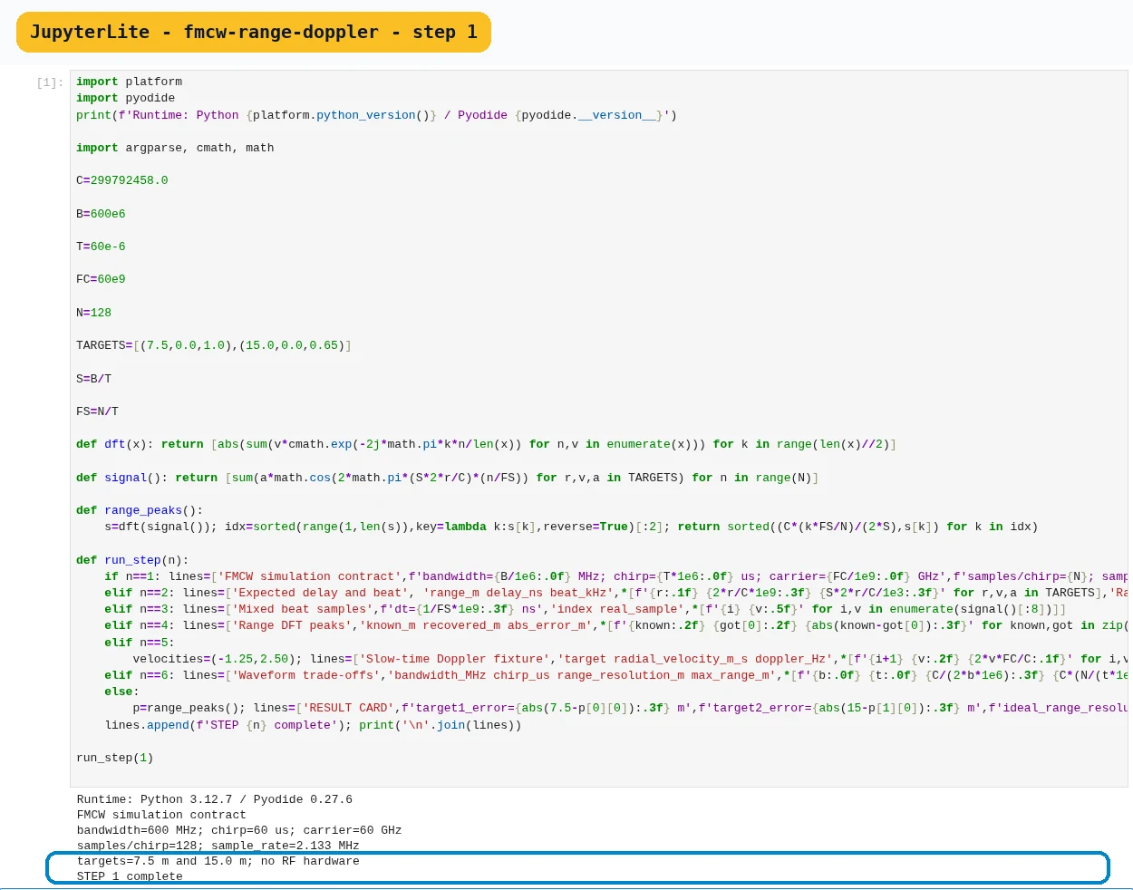
Step 1 · Python 3 in your browser (JupyterLite); numbered callout added to a real capture. Enlarge screenshot (new tab) Step 2
- Do
- Calculate delays and beat frequencies.
- You will see
- Each target's delay and expected beat frequency appear with units.
- Why it matters
- A target at range R creates an approximate round-trip delay of 2R/c.

Step 2 · Python 3 in your browser (JupyterLite); numbered callout added to a real capture. Enlarge screenshot (new tab) Step 3
- Do
- Generate one mixed beat signal.
- You will see
- The first eight real samples and their time spacing are printed.
- Why it matters
- Mixing transmit and receive signals produces a beat frequency linked to delay and range.
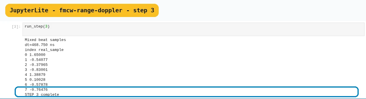
Step 3 · Python 3 in your browser (JupyterLite); numbered callout added to a real capture. Enlarge screenshot (new tab) Step 4
- Do
- Run a range DFT.
- You will see
- The two strongest bins recover target ranges with absolute error.
- Why it matters
- Samples within one chirp form range bins.

Step 4 · Python 3 in your browser (JupyterLite); numbered callout added to a real capture. Enlarge screenshot (new tab) Step 5
- Do
- Compare phase across chirps.
- You will see
- A slow-time DFT reports radial-velocity bins for both targets.
- Why it matters
- Doppler resolution improves with a longer coherent observation, while frame rate and target change limit how long samples remain comparable.

Step 5 · Python 3 in your browser (JupyterLite); numbered callout added to a real capture. Enlarge screenshot (new tab) Step 6
- Do
- Change bandwidth and chirp time.
- You will see
- The table shows range resolution and unambiguous-range changes.
- Why it matters
- Ideal range resolution is approximately c divided by twice the swept bandwidth, so more bandwidth separates closer reflectors.
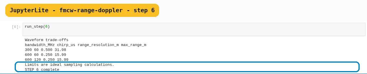
Step 6 · Python 3 in your browser (JupyterLite); numbered callout added to a real capture. Enlarge screenshot (new tab) Step 7
- Do
- Write a bounded result card.
- You will see
- The final card lists recovered errors and missing hardware evidence.
- Why it matters
- Synthetic chirps verify maths and code, not mmWave hardware, antennas, or a deployed scene.

Step 7 · Python 3 in your browser (JupyterLite); numbered callout added to a real capture. Enlarge screenshot (new tab)
Chapter checks
These questions refer to the chapter’s examples. Use the return links to review their answers.
What mainly improves ideal FMCW range resolution?
Return to the chapter’s knowledge checkWhich sample dimension supplies Doppler evidence?
Return to the chapter’s knowledge check
Return to FMCW mmWave Radar: Range, Doppler, and Angle · Browse Labs