8 PID Tuning and Applications
8.1 Start With a Safe Test Change
Tuning is not a hunt for perfect numbers. It is a controlled experiment where one change to the controller produces evidence about overshoot, settling time, oscillation, or sluggish response.
That matters because IoT loops often touch equipment, rooms, fluids, motors, and batteries. Start with a safe test condition and one adjustment you can undo. The right tuning method is the one that improves behavior without hiding risk from operators.

Phoebe’s Why
This chapter’s own numbers – Ku, Tu, sample period – describe the control loop itself, but a remote or wireless-actuated loop like the cold-room valve in the acceptance-record example also has a radio carrying its setpoint and status, and that radio has its own physics. Antenna gain in dBi is not amplification; it is focus, squeezing a fixed radiated power into a narrower pattern instead of spreading it over the whole sphere. Regulators cap the combination of conducted power and antenna gain as EIRP, so a more focused antenna must transmit at lower conducted power to sit under the same ceiling – the same “gain trades coverage angle for range” trade that a P-only loop makes when a tighter response in one operating region gives up margin somewhere else.
The Derivation
An isotropic radiator spreads transmit power \(P_t\) evenly over a sphere of radius \(d\):
\[S = \frac{P_t}{4\pi d^2}\]
A directional antenna concentrates that same power by a gain factor \(G\) into a narrower solid angle:
\[S_{directional} = G\,\frac{P_t}{4\pi d^2}\]
Regulators cap the combination in dB terms as EIRP:
\[\mathrm{EIRP(dBm)} = P_t(\mathrm{dBm}) + G(\mathrm{dBi})\]
Directivity relates to the beam’s angular width, so more gain means a narrower covered angle:
\[G \approx \frac{41253}{\theta_E\,\theta_H}\ \ (\theta\ \text{in degrees, symmetric beam }\theta_E=\theta_H=\theta)\]
Worked Numbers: A Remote Valve Actuator’s Link Budget
The chapter names no radio, so the worked numbers use a catalog-typical 2.4 GHz ISM license-exempt ceiling of 20 dBm EIRP:
- Omni reference antenna (0 dBi): to reach the 20 dBm EIRP ceiling, \(P_t = 20 - 0 = 20\) dBm \(= 100\) mW conducted
- 6 dBi directional patch: \(P_t = 20 - 6 = 14\) dBm \(= 10^{14/10} = 25.1\) mW conducted – the same regulatory range for \(100/25.1 = 3.98\times\) less RF-stage power
- Coverage angle paid for that gain: \(\theta = \sqrt{41253/10^{6/10}} = \sqrt{41253/3.98} \approx 102^{\circ}\) – the 6 dBi patch reaches the same EIRP-limited range only inside a roughly 102-degree beam, not the full sphere an isotropic radiator covers
A directional link saves conducted power (and battery current) at a fixed EIRP ceiling, but only while the valve stays inside that beam. If the actuator or gateway ever moves or gets reoriented during a retrofit, the acceptance record needs a retest, the same way a gain schedule needs a retest when the process moves to a different operating region.
8.2 Learning Objectives
By the end of this chapter, you will be able to:
- Plan a PID tuning session with safe limits, test signals, and rollback criteria.
- Use manual tuning and Ziegler-Nichols style tests as starting methods, not final proof.
- Diagnose response symptoms such as offset, oscillation, overshoot, sluggishness, saturation, and noisy command output.
- Match P, PI, PD, or PID configurations to application dynamics and measurement quality.
- Document tuning records so later changes can be checked without guesswork.
Core concept: Tuning changes controller behavior, but the process response decides whether the change is acceptable.
Why it matters: A loop that looks fast during one setpoint step may fail during a disturbance, actuator limit, sensor dropout, or operating-point change.
Key takeaway: Start conservative, add only the terms needed by measured response, test disturbance and recovery behavior, and keep a tuning record with the conditions that produced the approved gains.
8.3 Prerequisites
Before this chapter, revisit:
- PID Control Theory: P, I, and D term behavior.
- PID Control Fundamentals: loop signals and mode selection.
- Integral and Derivative Control: windup, damping, derivative filtering, and PI/PD/PID choice.
- PID Implementation and Labs: sampled implementation, output limits, and term logs.
8.4 What Tuning Changes
Tuning chooses controller gains and supporting limits so the closed loop behaves well for the real application. The gains are only part of the decision; sample period, output clamps, anti-windup, derivative filtering, sensor placement, and fallback behavior must be checked together.
P gain
Raises immediate correction. Too little gives sluggish response or offset. Too much produces overshoot, ringing, or instability.
I gain
Removes persistent offset. Too much causes slow oscillation, windup, and long recovery after saturation.
D gain
Adds damping from a rate estimate. Too much amplifies measurement noise or creates command spikes after setpoint changes.
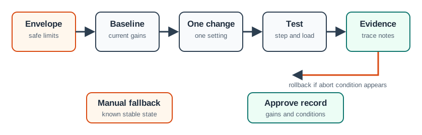
8.5 Tuning Session Safety
Tune only when the loop has clear boundaries. If a test can damage equipment, spoil product, or create an unsafe state, do not perform an aggressive oscillation test on the production loop. Use a model, lab rig, limited-output test, or supervised maintenance window.
- Define the test envelope. Record safe setpoint range, output range, maximum ramp, abort condition, and manual fallback.
- Start from a known state. Reset or record integrator state, current gains, operating point, and actuator limits.
- Change one thing at a time. Adjust P, I, D, filter, or limit settings separately unless a documented method requires a paired change.
- Capture response records. Save setpoint, process variable, output, saturation state, alarm state, sample period, and notes about disturbances.
- Approve by behavior. Gains are accepted only after setpoint and disturbance tests remain stable inside the operating envelope.
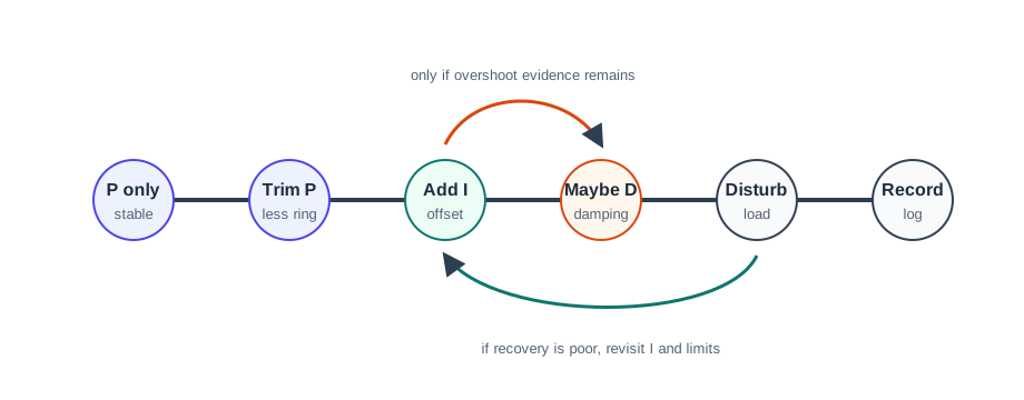
8.6 Manual Tuning Route
Manual tuning is useful when the process can be tested safely and when the team needs to understand how the loop reacts. It is slower than auto-tune but produces useful intuition and records.
- Begin with P only. Set I and D to zero or disabled, then raise P until response is useful but still stable.
- Reduce P if ringing appears. Keep a margin below the gain that causes sustained oscillation.
- Add I only for offset. Increase integral action gradually until persistent offset is removed without slow cycling.
- Add D only for overshoot or approach speed. Use filtered derivative on measurement when possible, and verify command noise.
- Retest under disturbance. A setpoint step is not enough; load and disturbance rejection must also be checked.
A very fast setpoint step can hide poor disturbance rejection, output chatter, windup, or measurement-noise sensitivity. Production tuning should favor repeatable stable behavior over the most dramatic trace in a single test.
8.7 Ziegler-Nichols As a Starting Method
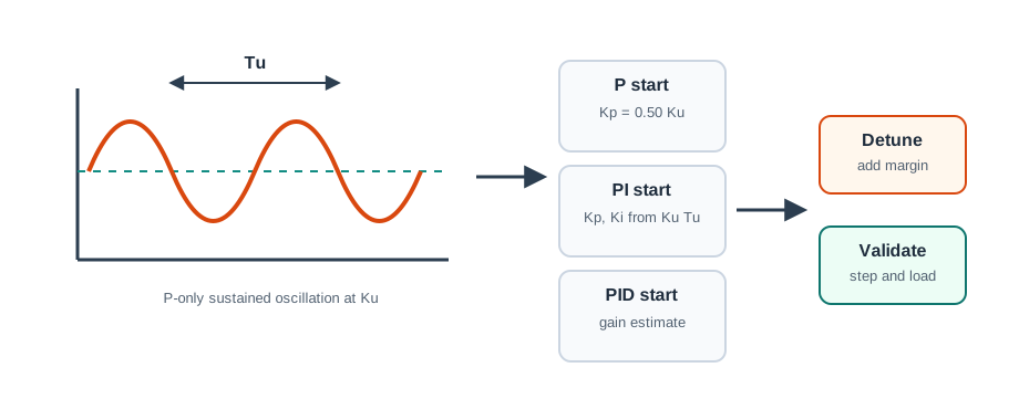
The classic closed-loop Ziegler-Nichols method raises proportional gain until the loop reaches sustained oscillation. That gain is the ultimate gain Ku; the oscillation period is Tu. Common formulas then produce aggressive starting gains.
P:   Kp = 0.50 * Ku
PI:  Kp = 0.45 * Ku,  Ki = 0.54 * Ku / Tu
PID: Kp = 0.60 * Ku,  Ki = 1.20 * Ku / Tu,  Kd = 0.075 * Ku * Tu
These values are not a deployment certificate. They are a starting point that usually needs detuning, anti-windup checks, derivative filtering, and disturbance testing.
Use when
The process can safely tolerate a controlled oscillation test, and the team needs a repeatable first estimate.
Avoid when
Oscillation could harm the process, actuator, product, or user. Use conservative step tests, model-based tuning, or lab characterization instead.
Check after
Check output saturation, windup recovery, derivative noise, setpoint kick, and behavior away from the test operating point.
8.8 Response Diagnosis
Good tuning work names the symptom before changing the gain. The same poor trace can have several causes, so look at setpoint, measurement, output, saturation, and timing together.
Persistent offset
Likely causes include too little integral action, actuator bias, unmeasured disturbance, or output clamp. Add I only after checking limits.
Fast oscillation
Often too much P or excessive delay. Reduce P, check sample period, and check whether the actuator is responding late.
Slow cycling
Often too much I or windup. Reduce integral action, add anti-windup, and check reset behavior after saturation.
Overshoot
May need lower P, slower setpoint ramp, derivative damping, or actuator limit changes. Do not add D if the measurement is too noisy.
Command chatter
Often derivative noise, quantized measurement, or too-short sample period. Filter the rate estimate and set command deadband if appropriate.
Good setpoint, poor disturbance
Retune for load rejection, not only setpoint tracking. Disturbance tests are part of the acceptance proof.
8.9 Application Patterns
Application context changes what “good” means. A thermal loop may accept slow settling if it avoids overshoot. A position loop may need damping and fast recovery. A level loop may prioritize avoiding overflow and actuator cycling.
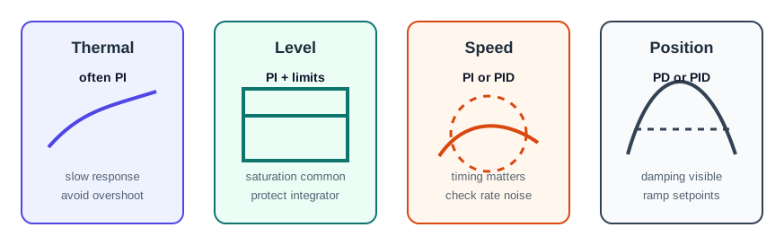
Thermal loops
Often slow, delayed, and naturally damped. PI is common; derivative is useful only when the measurement path gives a stable rate estimate.
Level or pressure loops
Disturbance rejection and actuator limits matter. Integral action needs anti-windup because valves and pumps often saturate.
Speed loops
Require quicker response and careful sample timing. Derivative or feedforward may help when measurement noise is controlled.
Position loops
Overshoot and ringing are visible. Damping, output limits, ramped setpoints, and mechanical backlash checks are usually important.
8.10 Operating Points and Gain Scheduling
One set of gains may not work everywhere. A process can be gentle near one operating point and sensitive near another. When the response shape changes across the allowed range, use conservative global gains or a documented gain schedule.
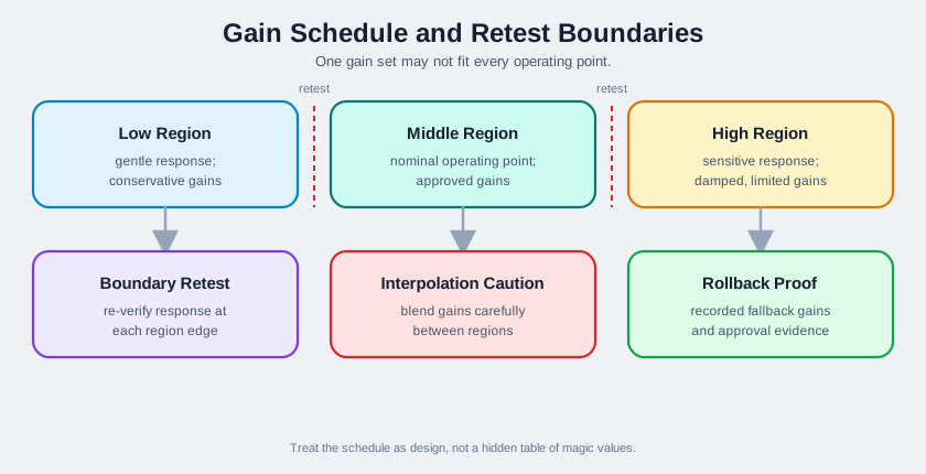
A gain schedule should be treated as part of the controller design, not as a hidden table of magic values. Record region boundaries, transition behavior, fallback gains, and the proof used to approve each region.
8.11 Tuning Decision Record
Each accepted tuning change should leave a decision record. The record does not need to be long, but it must be enough for another engineer to understand what was changed and why.
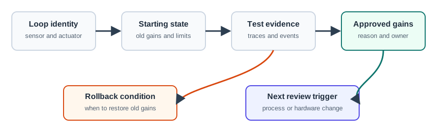
- Loop identity. Controlled variable, actuator, sensor location, sample period, output limits, and controller mode.
- Starting state. Previous gains, integrator handling, filters, setpoint, operating point, and known disturbances.
- Test proof. Setpoint trace, disturbance trace, output trace, saturation periods, alarms, and manual interventions.
- Decision. Approved gains, rejected gains, reason for acceptance, rollback condition, and next retest trigger.
8.12 Knowledge Check
8.13 Match the Tuning Records
8.14 Order the Tuning Decision
Key Concepts
- Manual tuning: Stepwise adjustment of P, I, and D terms while observing measured response.
- Ultimate gain: The P-only gain at which a safe test produces sustained oscillation.
- Ultimate period: The measured period between oscillation peaks at the ultimate gain.
- Conservative detuning: Reducing aggressive starting gains to improve stability, noise tolerance, and disturbance recovery.
- Disturbance rejection: The loop’s ability to recover when a load or environment change pushes the process away from its target.
- Gain scheduling: Using different gain sets for different operating regions when one gain set cannot handle the full range.
- Tuning record: A durable note containing gains, test conditions, proof, approval reason, and rollback trigger.
Common Pitfalls
Using Ziegler-Nichols as final proof
The method gives starting gains. It does not replace conservative detuning, anti-windup checks, and disturbance testing.
Tuning only at one operating point
Loops can behave differently at low, middle, and high output. Retest where process gain, delay, or actuator authority changes.
Ignoring actuator saturation
If the actuator is clamped, the integrator may keep accumulating. Saturation and recovery proof must be part of the tuning record.
Adding derivative to noisy measurements
Damping requires a trustworthy rate estimate. If rate noise dominates the command, use PI, filtering, setpoint shaping, or sensor improvements.
Changing gains without a rollback path
Production tuning needs previous gains, abort criteria, and a way to return to a known stable state.
Keeping undocumented magic numbers
Future maintainers need to know the condition that justified each gain. A short decision record prevents guesswork later.
8.15 Overview: Tuning Is Acceptance Proof
A tuned loop is not accepted because the gain values look reasonable. It is accepted because measured behavior stays inside the agreed envelope during the cases the application actually cares about: setpoint changes, disturbances, saturation, fallback, and recovery.
That makes tuning a proof process. Every accepted change should connect a symptom to a term, a term to a recorded response, and the recorded response to an operating decision. Without that chain, the numbers become private lore that the next maintainer cannot safely reuse.
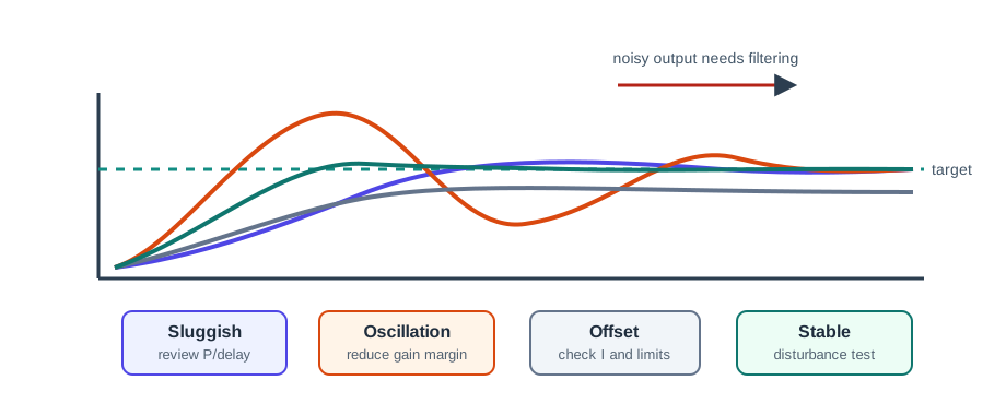
Small-screen read: approve gains only when recorded response covers the symptom, limit, disturbance, and recovery behavior the application must survive.
8.16 Tuning Acceptance Record
Before a gain change leaves the lab, write the acceptance record in the same language an operator or reviewer can inspect. Keep it short, but require enough evidence to explain why the loop is safer, steadier, or more useful than before.
Accepted Behavior
Record the approved overshoot, settling time, offset, cycling, command noise, saturation duration, and disturbance recovery target.
Rejected Behavior
Record the gain set or controller mode that failed, the symptom it caused, and the rollback state that was restored.
Retest Boundary
Record the operating point, load range, sensor condition, actuator limit, and process change that require the gains to be rechecked.
A strong record says, for example, “PI accepted for the cold-room valve at 30-70% load; retest required if valve travel changes, sample period changes, or recovery from door-open disturbance exceeds the approved trace.”
8.17 Single Traces Can Overfit
A gain set can look excellent on one step test because the operating point, disturbance shape, actuator authority, and sensor noise happen to match that run. The same gains can become fragile when the process moves to a different load, delay, or saturation condition.
This is why production tuning uses conservative approval. The accepted gains should have margin against noise, delay, output clamps, and expected disturbances. If the process behaves differently across regions, a gain schedule needs transition proof; if the proof is not available, conservative global gains are usually safer than a hidden table that only worked once.
8.18 Summary
PID tuning is a controlled decision process. Start with safe limits, tune from measured behavior, add integral and derivative action only when the response calls for them, test disturbance recovery, and keep the simplest stable configuration that satisfies the application.
8.19 See Also
- PID Control Theory: term behavior and response shape.
- Integral and Derivative Control: windup protection and derivative damping.
- PID Implementation and Labs: sampled implementation and term logs.
- Open-Loop and Closed-Loop Systems: feedback placement and fallback behavior.
8.20 What’s Next
The next chapter, Processes and Systems: PID Control, connects PID tuning back to broader process-control structure and system-level checks.