7  Lab: PID Implementation

7.1 Start With One Sampled Decision

A PID implementation is a repeated promise: read the process value, compare it with the setpoint, compute the output, and apply that output for one sampling interval. The controller is only as good as that small decision repeated reliably.

For IoT deployments, the story includes clocks, noisy sensors, actuator limits, and restart behavior. Start with a single sample step on paper, then decide what state must be remembered so the next step does not surprise the physical system.

In 60 Seconds

PID implementation is the discipline of turning control math into a timed software loop. A good lab proves the sample period, controller state, output limits, anti-windup behavior, derivative filtering, fallback rules, and term logs before the loop is trusted with a physical actuator.

7.2 Learning Objectives

By the end of this chapter, you will be able to:

• Translate continuous PID ideas into a sampled controller loop.
• Identify the state variables a controller must store between samples.
• Apply output limiting and anti-windup behavior without hiding actuator saturation.
• Decide when derivative filtering is required and when the D term should be omitted.
• Build lab proof that compares P, PI, and PID behavior without relying on brittle gain recipes.

PID Implementation Boundaries

MVU: Minimum Viable Understanding

Core concept: A digital PID controller is a scheduled state machine, not just a formula.

Why it matters: Timing jitter, stale measurements, actuator limits, and unbounded accumulation can make correct-looking code behave badly.

Key takeaway: Implement the loop in layers: validate signals, fix timing, clamp output, protect the integral term, filter derivative action, then tune from recorded term behavior.

7.3 Prerequisites

Before this chapter, revisit:

• Feedback Fundamentals: setpoint, process variable, error, and feedback direction.
• PID Control Fundamentals: P, I, and D term roles.
• Open-Loop and Closed-Loop Systems: when feedback should change the next command.

7.4 Implementation Boundary

An implementation boundary check should separate the physical process from the controller code. The controller receives a measured value, keeps a small amount of state, and returns a bounded command.

The boundary prevents two common mistakes. First, it stops the team from hiding process assumptions inside gain values. Second, it makes proof repeatable because another engineer can see which values came from sensors, which values were stored by the controller, and which values were sent to the actuator.

• Inputs: setpoint, measured process variable, validity flag, and timestamp.
• Stored state: previous error, integral accumulator, filtered derivative estimate, last output, and last sample time.
• Outputs: bounded command, saturation flag, mode state, and diagnostic terms.
• Term log: trend records for setpoint, measurement, error, P term, I term, D term, output, and fallback state.

7.5 Sampled-Loop Structure

The controller should run on a declared sample period. The exact value depends on process dynamics and measurement behavior, so the chapter uses a timing-fit method rather than a universal number.

Figure 7.1: Sampled PID loop structure

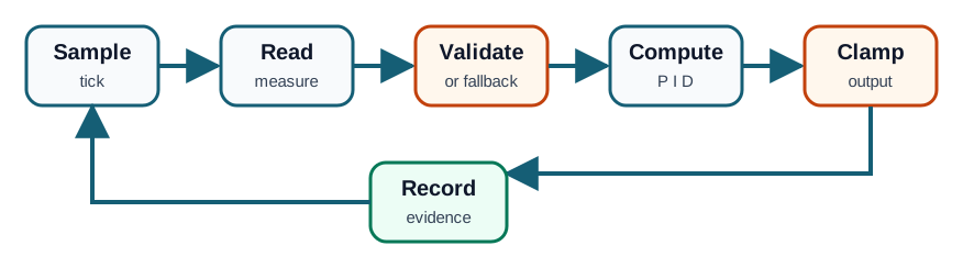
on each sample tick:
  measured = read_process_variable()
  if measured is invalid:
    command = fallback_command()
    record_fallback()
    return

  error = setpoint - measured
  proportional = Kp * error
  integral_candidate = integral + error * sample_period
  derivative_raw = (error - previous_error) / sample_period
  derivative = filter(derivative_raw)

  unconstrained = proportional + Ki * integral_candidate + Kd * derivative
  command = clamp(unconstrained, output_min, output_max)
  saturation = command != unconstrained

  integral = anti_windup_update(integral, integral_candidate, saturation, error, command)
  previous_error = error
  write_actuator(command)
  record_terms()

This structure makes the protection logic visible. If the measurement is invalid, the controller does not continue accumulating stale error. If the output saturates, the anti-windup policy decides whether the integral state should grow, stop, or be corrected.

7.6 Controller State

A stateless function cannot implement integral or derivative behavior correctly. The controller needs memory between samples.

Figure 7.2: PID controller state variables

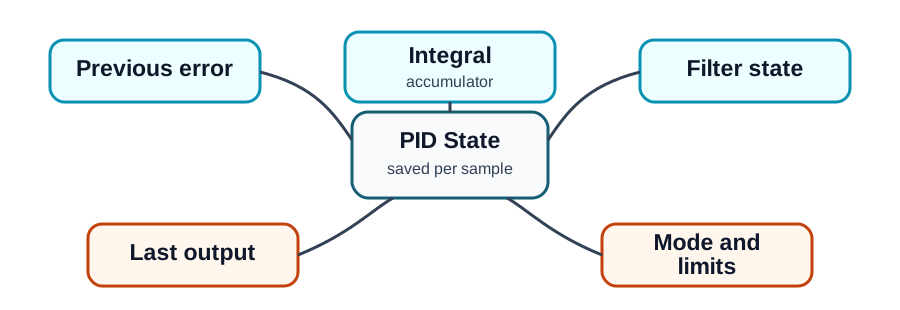
Previous Error

Supports the finite-difference estimate used by derivative action. It must be reset deliberately when the controller changes mode.

Integral Accumulator

Stores accumulated error. It needs a defined unit, a bounded range, and a policy for saturation and manual mode.

Filter State

Stores the smoothed derivative estimate or measurement-rate estimate. This state prevents one noisy sample from dominating the command.

Last Output

Supports bumpless transfer, rate limiting, and diagnostics when a command changes too sharply.

7.7 Output Limits and Anti-Windup

Every actuator has a physical range. PID code must clamp commands to that range and expose when clamping happened.

Figure 7.3: Anti-windup and output limiting

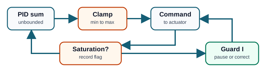
Anti-windup is not a tuning shortcut. It is a safety rule for what happens when the requested command is outside the actuator range.

Clamp First

Compute the unconstrained output, clamp it to the actuator range, and record whether saturation occurred.

Guard Accumulation

If the actuator is saturated and the error would drive it farther into saturation, pause or correct the integral update.

Support Recovery

When error changes direction or the actuator leaves saturation, allow integral action to resume so offset can be removed.

7.8 Derivative Filtering

The D term is useful only when the rate estimate is meaningful. If measurement noise dominates the rate estimate, derivative action becomes a command-noise amplifier.

Figure 7.4: Derivative filtering decision

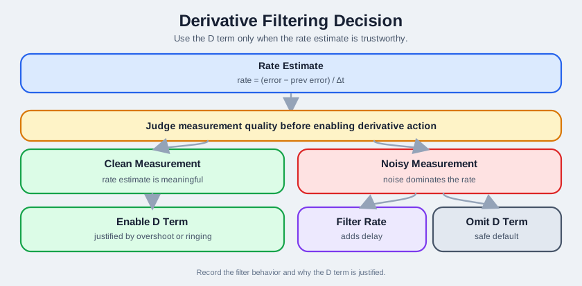
Use derivative action only after the lab shows that overshoot or ringing is a real problem and that the measurement path supports a stable rate estimate. Filtering can help, but filtering also adds delay. The implementation record should include both the filter behavior and the reason the D term is justified.

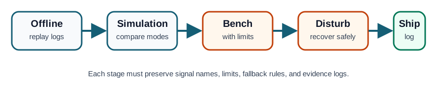
7.9 Lab Sequence

The lab should move from low-risk proof to higher-risk actuation. Do not begin with a live actuator if the timing, sign convention, and limits have not been proven.

Figure 7.5: PID implementation lab sequence

Run it: Do Lab 2 in the tuner below before you touch a real actuator. Pick a process model (slow thermal, medium motor, or fast flow), set the Test Mode to a setpoint step, and Run Response with P-only, then PI, then PID to watch each term change offset, overshoot, and settling. Switch the Test Mode to Step plus load disturbance to preview Lab 4, and use Apply ZN Estimate as a starting point you then refine from the recorded term behavior.

Lab 1: Offline Replay

Feed recorded measurements through the controller without writing to an actuator. Confirm sign convention, sample handling, term trends, output limits, and fallback behavior.

Lab 2: Software Simulation

Use a simple process model to compare P, PI, and PID behavior. The goal is not perfect realism; it is to expose term behavior before hardware risk.

Lab 3: Bench With Limits

Connect an actuator through conservative output limits. Verify saturation flags, anti-windup behavior, and manual override before increasing authority.

Lab 4: Disturbance Recovery

Apply a controlled disturbance and record how the loop recovers. Compare offset, overshoot, settling behavior, and actuator stress.

7.10 Simulation Run Addendum

Use simulation as run proof, not as final proof of field behavior. Every run should connect a question to a model boundary, one changed condition, and a decision about the next lab step.

Run it: Use the feedback-loop animation below to gather the term proof this addendum asks you to record. Raise Kp alone and watch the output move in the correct direction but hold a persistent offset, add Ki to see the offset removed, then push the Actuator limit with a Load step to watch integral windup and recovery. Finally raise Sensor noise and add Kd to confirm the D term only adds useful damping when the measured rate is trustworthy, not when noise dominates.

Simulation item	Proof to record
Run question	Offset, overshoot, oscillation, saturation, disturbance response, fallback, or sample-timing behavior under inspection.
Model boundary	Controlled result, measured result, actuator command, process response, output limits, sample timing, planned disturbance, and excluded real-world effects.
Term proof	P moves the result in the correct direction; I removes persistent offset with anti-windup; D adds damping only when measurement rate is trustworthy.
Run plan	Baseline, P-only, PI, candidate PD or PID, disturbance check, limit check, and one changed item per run.
Decision record	Trace observations, command observations, saturation and recovery behavior, keep or reject decision, and next bench or field proof needed.

Simulation can support a design direction. It cannot prove safety, wiring, actuator wear, sensor faults, network delay, or operator behavior without later representative field proof.

7.11 Controller Log Template

An implementation lab should produce records, not just screenshots. At minimum, capture a time series with the fields below.

Signals

• Time and sample index.
• Setpoint and measured value.
• Error and sign convention.
• Measurement validity.

Terms

• P contribution.
• I contribution and accumulator value.
• D contribution and filter state.
• Unconstrained output.

Protection

• Clamped output.
• Saturation flag.
• Fallback mode.
• Manual/automatic state.

Outcome

• Offset after settling.
• Overshoot or ringing.
• Recovery after disturbance.
• Actuator cycling or rate limit events.

7.12 Implementation Readiness Checklist

Before deployment, the implementation record should answer these questions with proof:

• Does the controller run only on the declared sample tick?
• Does the code reject invalid or stale measurements before updating PID state?
• Are output limits applied before anti-windup logic?
• Is integral state bounded, resettable, and included in diagnostics?
• Is derivative action filtered or deliberately omitted?
• Does manual-to-automatic transfer avoid a sudden output jump?
• Does the controller log show P, I, D, output, saturation, and fallback state?

7.13 Knowledge Check

Choose the Safer Implementation Step

Match the Implementation Concepts

Order the Implementation Check

Key Concepts

• Sample period: The scheduled interval between controller calculations.
• Controller state: Stored values such as previous error, integral accumulator, filter state, last output, and mode.
• Output clamping: Limiting the calculated command to the actuator’s allowed range.
• Anti-windup: Logic that prevents the integral state from growing in a harmful direction during saturation.
• Derivative filtering: Smoothing a rate estimate so measurement variation does not dominate the command.
• Bumpless transfer: Switching between manual and automatic modes without a sudden output jump.
• Controller log: Time-series records that show signals, terms, limits, flags, and outcomes.

7.14 Common Pitfalls

Timing Hidden in the Main Loop

If PID code runs whenever other tasks happen to finish, the I and D terms no longer match the assumed sample period.

Integral Growth During Saturation

If the output is clamped but the accumulator keeps growing in the same direction, the loop can overshoot after the process finally responds.

Derivative on Untrusted Data

If measurements jump because of noise or stale reads, derivative action can create command spikes instead of damping.

Tuning Without Term Logs

If only the final output is recorded, maintainers cannot tell whether the response came from P action, accumulated I action, D action, or saturation.

7.15 Implementation as State Contract

A PID implementation is a contract about what state the controller is allowed to remember and when that state is allowed to change. The formula is only the center of the loop. The surrounding contract declares sample timing, valid inputs, stored terms, output limits, fallback mode, and the records that prove each update was legal.

This matters because most live PID failures do not look like a wrong equation. They look like stale measurements updating the integral term, a noisy derivative estimate commanding spikes, a saturated actuator hiding windup, or a manual-to-automatic transfer that jumps because old state was reused without a reset rule.

The boundary diagram keeps implementation proof honest: inputs are validated before state changes, controller memory is explicit, limits convert requested output into a safe command, and the evidence log explains the next sample instead of leaving behavior hidden inside gains.

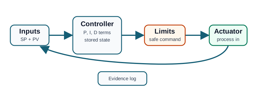
Small-screen read: each PID update should prove valid inputs, stored state, bounded output, actuator command, and evidence before the next sample changes memory.

7.16 Prove Lab Trace Before Authority

Before giving a controller full actuator authority, require a trace that shows why each command was produced. A good trace lets a reviewer replay the decision, not just admire a smooth output curve.

Timing Proof

Sample index, timestamp, expected period, measured period, missed-tick handling, and whether the update was skipped or applied.

State Proof

Previous error, integral accumulator, derivative filter state, mode, saturation flag, and reset reason after fallback or manual transfer.

Authority Proof

Unconstrained command, clamped command, actuator limit, rate limit, fallback command, and the exact condition that allowed higher authority.

The release question is not “did the test look stable?” It is “can another engineer explain every command from the recorded inputs, state, limits, and mode transitions?”

7.17 State Debt Survives Sampling

Proportional action mostly reacts to the current error. Integral and derivative behavior carry memory across samples. That memory is useful only while its assumptions remain true. When the sensor is stale, the actuator is saturated, the mode changes, or the sample period slips, stored state can become debt that appears later as overshoot, command spikes, or slow recovery.

Anti-windup, derivative filtering, bumpless transfer, and fallback reset rules are all ways of managing stored state debt. They do not make tuning optional. They make tuning reviewable because the controller can show when it trusted state, froze state, reset state, or refused to update state.

7.18 Summary

PID implementation is a software and traceability problem. A durable controller has a declared sample period, explicit state, bounded output, anti-windup behavior, derivative filtering or an explicit decision to omit D, fallback handling, and logs that expose the controller terms. The lab sequence should prove those details before the controller receives full actuator authority.

7.19 See Also

• PID Control Fundamentals
• Feedback Fundamentals
• Actuators
• Control Gateways

7.20 What’s Next

Continue with Integral and Derivative Control to examine accumulated error, windup protection, derivative damping, and when full PID is worth the added complexity.