Chapters

3 Sensor Hardware Selection

sensors
applications
hardware

3.1 Start With the Hardware Story

Picture a cold room that must warn staff before food warms too far. A sensor board may fit the plug and still read the warm case around itself instead of the air beside the food.

Name the thing to measure first. Add its useful range, the place of the sensor, the needed change in reading, and the action that follows. Then look for hardware that can keep that claim after it is mounted.

Check the whole installed path. Power, wiring, moisture, heat, airflow, case shape, and service access can all alter the result. A cheap part may need costly care. A precise part may fail in the wrong place.

This cold-room story cannot choose one sensor for every job. It does not prove life, calibration, interface fit, or safe maintenance. Those claims need an installed test and a retest rule.

Use the Practitioner sections to build the hardware choice record. Use Under the Hood for sensing physics, interfaces, error, and power. The deeper work explains why the simple measurement claim must remain visible.

Walk the cold-room choice. Name the product. Name the air zone. Name the safe limit. Name the alarm time. Name the staff action. Mark the coldest place. Mark the warmest place. Mark the door. Mark the fans. Mark the drain. Mark the service path.

Try the first sensor. Read its range. Read its error. Read its useful step. Read its response time. Read its power need. Read its link type. Read its case limit. Read its care rule. Do not stop at the plug shape.

Place it in the open. Compare a known meter. Change the air slowly. Change it fast. Open the door. Close the door. Start a fan. Stop a fan. Add moisture. Add ice. Warm the case. Move the probe. Record every change.

Check the wire and link. Bend the cable. Pull the plug. Add noise. Lose the local link. Restore it. Swap two ports. Check the sensor name. Check the unit. Check the time. Check old data. Check repeated data. Keep the alarm safe.

Check power. Start cold. Start warm. Lower the supply. Lose power. Restore power. Measure wake time. Measure steady use. Measure send use. Check the first reading. Check the last saved state. Make low power visible.

Check care. Can staff find it? Can they clean it? Can they remove it? Can they fit a spare? Can they prove the new name? Can they run the known check? Can they record the result? Can they avoid the food area?

Check drift. Compare at day one. Compare after a month. Compare after a move. Compare after wash. Compare after ice. Set a clear limit. Set a retest date. Set a retest cause. Reject a reading outside proof.

Compare two parts fairly. Use the same place. Use the same known meter. Use the same time. Use the same power. Use the same case. Count part cost. Count fitting cost. Count care cost. Count false alarms. Count missed alarms. Keep the best whole fit.

Close the record. Keep the true measure. Keep the range. Keep the place. Keep the error. Keep the test. Keep the owner. Keep the spare. Keep the retest rule. State what is not proven. A selected part is still a field claim.

Start with the job the hardware must survive: where it sits, what it touches, how it is powered, and what would make its reading untrustworthy. A sensor part becomes a selection only when that story is recorded as evidence.

Hardware Selection Starts With a Measurement Claim

Sensor hardware selection is the claim that a physical device can observe the right condition, in the right place, with enough quality for the application decision. A shopping list is not a selection record. The selection must connect the measurement need, installed environment, interface, power behavior, calibration plan, maintenance access, and validation evidence.

The useful question is not "which sensor is best?" The useful question is what the application must prove and which hardware can preserve that evidence after it is mounted, powered, wired, calibrated, and maintained in the field.

Worked example. Suppose a cold-room monitor must alert when product-area air temperature exceeds 8 °C for more than five minutes. A convenient board-mounted temperature sensor inside a sealed node may be easy to wire, but it measures enclosure temperature, not product-area air. A better selection claim names the measurand (air temperature near stored goods), range (0–15 °C), useful resolution (for example 0.5 °C if the decision threshold is 8 °C), placement, cable or probe route, condensation risk, calibration comparison, and retest trigger after relocation or enclosure change. Without those facts, the hardware is only compatible with the controller, not proven for the application decision.

If you only need the intuition, use this rule: approve sensor hardware only when the selected device fits the measurand, placement, interface, environment, data-quality checks, maintenance plan, known limit, and retest trigger.
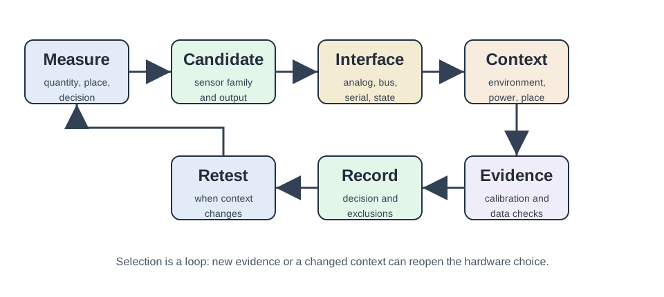
Before accepting a compatible part, inspect Figure 3.1 to see how the measurement claim constrains every later choice. The diagram is a review loop because field evidence can force the team back to the need rather than merely confirming the first candidate.

Sensor hardware selection flow from measurement need through candidate, interface, context, evidence, record, retest, and revised measurement claim.
Figure 3.1: Sensor hardware selection loop from measurement need through evidence and retest

Read Figure 3.1 from the measurement need to the candidate family, then check the interface and installation context together. Evidence from placement, power, calibration, and data quality enters the decision record before a device is accepted. The retest trigger closes the loop: if the context or evidence changes, the hardware claim must be revised. This is how the chapter separates an electrically convenient module from a defensible field selection.

Measurement Fit

Name the quantity, location, expected range, meaningful resolution, response behavior, and decision that depends on the reading.

Interface Fit

Check analog, digital, pulse, I2C, SPI, UART, 1-Wire, GPIO, timing, bus length, address, reference, and parsing assumptions.

Evidence Fit

Keep calibration, reference comparison, plausibility checks, noise, drift, saturation, missing values, and quality-state behavior visible.

Lifecycle Fit

Review power, enclosure, mounting, cleaning, replacement, firmware, ownership, and what field change reopens the hardware decision.

Worked example. "Light sensor" is not a measurement claim; photoresistors, photodiodes, and phototransistors are three different transducer families that happen to share a name. A photoresistor (LDR) is built from a cadmium-sulfide cell whose resistance falls as light rises -- roughly 106 Ω in darkness down to about 10 Ω in bright sunlight -- which is cheap and simple but only tells you a relative light level, not a calibrated illuminance. A photodiode instead turns light directly into a current, trading that simplicity for a faster, more linear response the interface has to condition properly. Naming which family a "light sensor" candidate actually is, and why, belongs in the measurement-fit claim before a part number is chosen.

3.1.1 Light Measurement Before Part Selection

The three common light units describe different parts of one geometry. Figure 3.2 starts with a 120-candela spotlight, preserves flux through its cone, and compares illuminance on near and far surfaces.

A lamp cone distinguishes candela intensity, lumen flux and surface lux. Doubling distance quarters illuminance; surface tilt reduces it further.
Figure 3.2: A spotlight cone separates candela intensity, lumen flux, and lux on near and far target surfaces.

In Figure 3.2, Candela · cd belongs to the lamp’s selected direction, while Lumen · lm totals flux across the 0.84 sr cone. The near surface reads 120 lx at 1 m; the far surface reads 30 lx at 2 m, and a 60° tilt halves that result again through the cosine term.

Before comparing light-sensor parts, name the photometric quantity the application needs. The three common units describe different points along the path from a source to a receiving surface.

QuantitySymbol and unitWhat it saysTypical question
Luminous intensityIvI_v, candela (cd)Visible-light strength in one direction; 1 cd=1 lm/sr1\ \mathrm{cd}=1\ \mathrm{lm/sr}How strong is the source along this viewing direction?
Luminous fluxΦv\Phi_v, lumen (lm)Total visible-light output carried through a solid angleHow much eye-weighted light leaves the lamp or beam?
IlluminanceEvE_v, lux (lx)Flux arriving per unit area; 1 lx=1 lm/m21\ \mathrm{lx}=1\ \mathrm{lm/m^2}How much light reaches the desk, crop leaf, or sensor plane?

The bridge between intensity and flux is solid angle. If intensity is approximately uniform over a beam of solid angle Ω\Omega, then

Φv=ΩIv(θ,ϕ)dΩΦvIvΩ.\Phi_v = \int_{\Omega} I_v(\theta,\phi)\,d\Omega \quad\longrightarrow\quad \Phi_v \approx I_v\Omega.

A cone with half-angle α\alpha subtends Ω=2π(1cosα)\Omega=2\pi(1-\cos\alpha) steradians. An ideal isotropic source covers 4π4\pi steradians, so a uniform 100 cd100\ \mathrm{cd} source would emit 4π(100)1257 lm4\pi(100)\approx1257\ \mathrm{lm}. Real lamps are not isotropic: their intensity depends on direction, which is why a lumen rating alone cannot predict the reading at a particular sensor.

At the receiving surface, flux is spread over area:

Ev=dΦvdA.E_v=\frac{d\Phi_v}{dA}.

For a small source observed from distance rr, the same patch of solid angle covers an area proportional to r2r^2. Combining that geometry with the projected-area factor gives

Ev=Ivcosβr2,E_v=\frac{I_v\cos\beta}{r^2},

where β\beta is the angle between the arriving ray and the surface normal. Face the surface squarely toward the source and cosβ=1\cos\beta=1; tilt it and the same beam spreads over more effective area.

Walk the numbers. A source has intensity 100 cd100\ \mathrm{cd} toward a sensor mounted normally to the beam. At 1 m1\ \mathrm{m} the sensor receives 100/12=100 lx100/1^2=100\ \mathrm{lx}. At 3 m3\ \mathrm{m} it receives 100/3211.1 lx100/3^2\approx11.1\ \mathrm{lx}, not one third as much. Distance tripled, illuminated area grew ninefold, and illuminance fell by the same factor. If the sensor is also tilted by 6060^\circ, its reading falls to about 5.6 lx5.6\ \mathrm{lx} because cos60=0.5\cos60^\circ=0.5.

This distinction changes part selection. A lamp-output monitor may need flux or directional intensity data, while an automatic room-light controller needs calibrated illuminance at the occupied plane. A bare photodiode measures wavelength-dependent optical power, not lux by itself; a lux sensor adds a spectral response intended to approximate human photopic sensitivity. The hardware record must therefore state the measurand, spectrum, geometry, distance, orientation, optical cover, expected lux range, and calibration reference before comparing resolution or interface convenience.

Build the Hardware Decision Record

A hardware decision record captures why one candidate was accepted and why alternatives were rejected. It should be clear enough that another reviewer can repeat the reasoning after procurement, installation, maintenance, or replacement.

Selection Area
Evidence to Keep
Common Weak Point
Retest Trigger
Measurand and placement
Physical quantity, units, expected span, mounted location, enclosure influence, response need, and decision threshold.
The sensor is placed where wiring is easy instead of where it observes the condition the application needs.
Location, enclosure, airflow, target material, operating range, threshold, or application decision changes.
Interface and data path
Electrical interface, addressing, timing, reference voltage, bus length, sample rate, units, timestamps, and error states.
The controller can read values, but the record loses units, timing, source identity, or invalid-reading state.
Controller, firmware, bus layout, sample rate, parser, data schema, or gateway path changes.
Calibration and validation
Reference check, calibration date, adjustment, drift check, noise behavior, saturation limits, and field comparison result.
A factory setting or one bench reading is treated as proof for every environment and maintenance interval.
Sensor replacement, reference method, field condition, maintenance interval, firmware, or validation threshold changes.
Power and maintenance
Sleep behavior, warm-up or stabilization, duty cycle, service access, cleaning, replacement, diagnostics, and owner.
The device works once but cannot be powered, inspected, cleaned, recalibrated, diagnosed, or replaced in service.
Battery plan, power budget, enclosure, service access, cleaning need, ownership, or expected deployment life changes.

Rejected candidates are useful evidence. Record why a part was excluded: wrong measurand, narrow range, poor environmental fit, interface risk, weak placement, calibration burden, power cost, missing diagnostic state, or maintenance access. This prevents the same unsuitable option from returning later as an undocumented shortcut.

Sensor hardware decision record template Measurement claim: what physical condition must be measured, where, and for which application decision. Accepted hardware: sensor family or module, interface, controller path, placement, power mode, and enclosure assumptions. Accepted evidence: range, response, calibration or comparison, data quality checks, units, timestamp, validity state, maintenance access, and diagnostics. Known limit: the claim the selected hardware does not support, such as safety action, precise metrology, outdoor use, or unsupported placement. Owner: who maintains calibration, firmware, thresholds, cleaning, replacement, diagnostics, and documentation. Retest trigger: the exact sensor, placement, enclosure, interface, sample rate, threshold, environment, power, calibration, or decision change that reopens review.

Worked example. A wearable motion-capture node makes the interface and lifecycle rows concrete. The design requirements come first and drive the hardware, not the reverse: fully wireless, no external infrastructure such as fixed cameras, real-time and interactive, and easy enough to use that the technology becomes ordinary rather than a lab novelty. A node meeting that brief, such as the Orient-5 design, pairs two radios (Bluetooth at 2.5KB/s and a 2.4GHz link at 50KB/s) with an 8kHz gyroscope and 4kHz accelerometer, and reports fused quaternion orientation at 200Hz over Bluetooth or 2500Hz over the 2.4GHz link. That radio choice is itself a hardware decision with a lifecycle consequence: a TDMA-scheduled 2.4GHz deployment running twelve nodes can sustain a 128Hz update rate per node, but doubling to twenty-four nodes on the same shared link halves it to 64Hz. The accepted-evidence row should record which of those two operating points the application actually needs before more nodes get added to the network.

Hardware Fit Fails at Boundaries

Weak hardware decisions usually fail where the physical world meets the data path. A sensor may measure the right quantity but in the wrong location. It may have a convenient bus but lose units or error states. It may pass calibration in one condition but drift in another. It may draw more power after warm-up, stabilization, retries, or environmental stress than the node budget allows.

To make the boundary problem concrete, inspect Figure 3.3 before judging this device by connector or resolution alone. The photograph identifies the physical camera assembly; the key selection question is the kind of data that assembly produces and what the downstream path must preserve.

A black Prophesee event camera evaluation kit with a lens and ribbon-connected circuit boards
Figure 3.3: Dynamic Vision Sensor event-camera evaluation kit; photo by Auledas, CC BY 4.0

In Figure 3.3, start at the lens and camera body, then follow the ribbon connection into the processing boards. Unlike an ordinary frame camera, a Dynamic Vision Sensor reports changes in brightness as events, so timing, interface bandwidth, storage, and algorithms must accept an event stream. The hardware can be electrically compatible yet still be wrong for a frame-based application. That example connects physical fit to the evidence and service boundaries reviewed next.

Physical Boundary

Mounting, airflow, moisture, dust, vibration, sunlight, target material, enclosure, and mechanical stress decide what the sensor actually sees.

Electrical Boundary

Reference voltage, grounding, bus length, address conflicts, timing, shielding, and signal conditioning decide whether readings survive integration.

Evidence Boundary

Calibration, drift, noise, missing values, saturation, validity flags, timestamps, and comparison checks decide whether readings can support decisions.

Service Boundary

Cleaning, inspection, replacement, recalibration, firmware, diagnostics, and support ownership decide whether the choice remains trustworthy.

False confidence is common. A hardware module may produce stable numbers while sensing the enclosure temperature instead of room air. A digital interface may hide analog front-end noise. A low-power sensor may become high-cost when warm-up, radio retries, and frequent validation are included.

Worked example. A comfort sensor mounted in a sealed electronics box can read 29 °C while the room reference thermometer reads 22 °C, because the board, regulator, and radio warm the enclosure. The I2C transaction is still valid and the data may be smooth, but the physical boundary is wrong: the sensor is measuring self-heating plus trapped air. A defensible fix might move the probe into free airflow, add a vented shield, record an offset only if it remains stable against a reference, and retest whenever the enclosure, board power, sampling interval, or mounting location changes.

The under-the-hood rule is to ask what would make the selected hardware lie, go silent, drift, saturate, or become unserviceable. If that change would alter the application decision, it belongs in the decision record as a limit, diagnostic, fallback, or retest trigger.

Worked example. Clinical fall-risk assessment shows three very different hardware answers to the same measurement claim: how well can a person maintain postural balance? The CDC put the annual US cost of falls at roughly \$34 billion in 2013, projected to reach \$55 billion by 2020, which is why the hardware choice behind "measure balance" is not a minor detail. The current gold standards sit at opposite ends of the hardware trade-off: interview-and-observation tests (a timed sit-to-stand, a timed up-and-go walk, a single-leg stance) are cheap but subjective and non-repeatable, while gait-lab force plates with reflective motion-capture markers are objective but expensive equipment few clinics can install. Between those two, a Dynamic Vision Sensor (DVS) camera -- an event camera that reports pixel-level brightness changes at roughly 1µs resolution instead of full frames, a response profile researchers have likened to the visual cortex's V1 layer -- has been proposed as an off-body, non-contact candidate that integrates with an existing clinical workflow at a fraction of a force plate's cost (Nalci et al., IEEE EMBC 2015). The evidence-fit question for a hardware record is not "which sensor is most advanced" but which of these three known limits -- subjective and non-repeatable, objective but unaffordable at scale, or new enough that its clinical validation is still being built -- the application can actually live with.

Validate a Balance-Sensing Claim, Not Just the Camera

A DVS balance experiment becomes evidence only after its event stream is reduced to a repeatable motion measure and compared across controlled conditions. One useful summary is total event-motion variance over a fixed trial, normalized by the same declared reference so that trials remain comparable. Eyes-open, eyes-closed, and eyes-closed-with-haptic-feedback trials then test an expected ordering rather than merely producing three attractive traces: removing visual feedback should change sway evidence, while useful feedback should move the measure toward the accepted reference condition. Normalization helps comparison, but it does not remove the need to record trial duration, region of interest, distance, lighting, event thresholds, filtering, stance protocol, and missing or saturated events.

Repeat the protocol for left- and right-foot stance and retain per-participant results. A mean alone can hide a method that works for one stance side or a few participants but fails elsewhere. Side-to-side asymmetry may be a real characteristic of the person, a placement or occlusion effect, or processing bias; the validation record should not choose among those explanations without follow-up evidence. Report the distribution, paired differences, exclusions, and repeatability before claiming that the method generalizes.

A second sensor can test whether both systems preserve the same dynamics. Estimate power spectral density from synchronized DVS and balance-board signals using the same time interval and clearly documented preprocessing. Agreement in the frequency bands relevant to postural sway is stronger evidence than similar-looking time plots, because it checks where motion energy is distributed. Disagreement is diagnostic rather than automatically disqualifying: camera geometry, event noise, board calibration, filtering, sample timing, or genuinely different measured quantities can all change the spectra. Hardware acceptance therefore requires both discriminating conditions and agreement limits against a reference—not a single demonstration that the DVS produced data.

3.2 Summary

Sensor hardware selection begins with the measurement claim and application decision, not a shopping list. Work outward through the measurand, range, response, placement, environment, interface, power, calibration, data quality, and maintenance access needed to support that claim. A convenient interface does not prove measurement quality or field reliability, so preserve rejected candidates and the reasons for rejecting them. Reopen the review when the sensor, placement, enclosure, interface, sample rate, threshold, environment, power budget, calibration method, maintenance plan, or application decision changes.

3.3 Key Takeaway

Select sensor hardware by evidence fit. The accepted record should tie measurement need, physical placement, interface, calibration, data quality, maintenance owner, known limit, and retest trigger to the decision the application must support.

3.4 See Also

Sensor Applications: Domain Overview

Start with the domain, condition, context, decision, and evidence that shape the hardware choice.

Sensor Application Architecture

Place the selected hardware inside the node, gateway, processing, storage, quality-state, and action path.

Sensor Lab Workflow

Turn selection evidence into calibration, comparison, logging, and retest exercises.

Mobile Phone as a Sensor

Compare fixed hardware selection with phone-based sensing, permissions, placement, and context limits.