17 BLE in Python with Bleak
bluetooth-ble
bt
impl
python
Key Concepts
- bleak (Bluetooth Low Energy platform Agnostic Klient): Python async BLE library supporting Windows (WinRT), macOS (CoreBluetooth), and Linux (BlueZ) backends
- BleakClient: bleak class representing a connection to a BLE peripheral; provides methods for service discovery, read, write, start_notify, stop_notify
- BleakScanner: bleak class for BLE device discovery; supports filtering by service UUID, device name, and RSSI threshold
- asyncio.run(): Python coroutine runner; required for bleak operations which are all async; use asyncio.get_event_loop() for integration with existing async frameworks
- UUID String Format: bleak accepts both 16-bit UUIDs as “0000xxxx-0000-1000-8000-00805f9b34fb” (128-bit expanded form) and short “xxxx” strings; use full 128-bit format for custom services
- characteristic.properties: bleak property set of enabled operations: {‘read’, ‘write’, ‘notify’, ‘indicate’, ‘write-without-response’} — check before attempting operations
- client.start_notify(uuid, callback): Registers a Python callback function called when a BLE notification arrives; callback receives (sender_handle, bytearray_data)
- GATT Error Codes in bleak: BleakError wraps ATT error codes; common causes: device not paired (0x05), wrong UUID (0x01), characteristic not found (service discovery needed)
17.1 Minimum Viable Understanding
BLE development in Python centers on the bleak library, which provides cross-platform async APIs for scanning, connecting, and interacting with BLE devices. Production BLE applications need RSSI filtering for reliable device discovery, GATT service exploration for data access, and exponential smoothing for stable proximity detection – zone-based classification (immediate/near/far) is far more reliable than precise distance calculations due to inherent RSSI variability.
17.2 Learning Objectives
By the end of this chapter, you will be able to:
- Implement Production BLE Scanners: Configure device filtering by RSSI threshold and name patterns using the bleak library
- Analyze GATT Services: Connect to BLE devices and enumerate services and characteristics to assess device capabilities
- Distinguish Beacon Protocols: Compare iBeacon and Eddystone advertisement packet structures and justify protocol selection for a given use case
- Design Proximity Detection Systems: Apply RSSI smoothing algorithms and construct zone-based presence detection with exponential moving averages
- Develop Async BLE Applications: Construct event-driven Python programs using asyncio and diagnose disconnection handling for production reliability
Chapter Roadmap
Read this chapter as a Python BLE implementation path:
- First establish the Bleak role model, prerequisites, and scanner evidence you need before connecting to anything.
- Then inspect GATT services and beacon advertisements so UUIDs, properties, iBeacon fields, and Eddystone fields are explicit.
- Next turn noisy RSSI samples into proximity zones using thresholds, EMA smoothing, and the alpha trade-off.
- After that connect the scripts to deployment evidence: power choices, visual stack references, quizzes, and a retail analytics pattern.
- Finally review runtime boundaries, reconnection mistakes, common pitfalls, and next-step chapters before treating the script as production-ready.
Checkpoint callouts summarize what should be defensible before you continue; collapsed examples and galleries can be opened when you need implementation detail.
For Beginners: Python BLE Development
What you’ll learn: Production-ready Python implementations for common BLE tasks using the bleak library.
Prerequisites:
- Basic Python with asyncio understanding
- BLE concepts from Bluetooth Fundamentals
- Code examples from BLE Code Examples
Why Python for BLE? Python’s bleak library provides cross-platform BLE support (Windows, macOS, Linux) with clean async APIs, making it ideal for gateways, data collection, and prototyping.
Python BLE Implementation Pattern
Use Python BLE code where the device doing the Bluetooth work has enough compute, storage, and operating-system support to run a gateway or test tool.
- Start with scanning filters: service UUID, name pattern, and minimum RSSI.
- Connect only after you have selected a specific target from scan results.
- Discover services before reading or subscribing to characteristics.
- Treat RSSI distance as an estimate; classify broad zones instead of promising exact meters.
- Build reconnection handling from the first prototype because BLE links can drop normally.
In this pattern, the Python host is the BLE Central and GATT client. While scanning it is acting as an Observer; after selection it initiates the connection and reads, writes, or subscribes to the peripheral’s GATT server. If the product requirement says a phone must discover the Python process or read a characteristic served by it, that is a Peripheral/GATT-server requirement and belongs on firmware or a platform-specific stack, not plain Bleak.
17.3 Prerequisites
Before working through these implementations:
- BLE Code Examples and Simulators: Basic Python scanner and GATT concepts
- Python Environment: A currently supported Python version for your chosen
bleakrelease, installed withpip install bleak
17.4 BLE Scanner with Device Filtering
A production scanner with RSSI filtering and statistics:
Expected scanner output should include:
- The scan duration and minimum RSSI threshold, for example
15.0sand-70 dBm. - Each matching device name, address or platform identifier, latest RSSI, and rough distance estimate.
- A final count of devices that passed the filter.
- Per-device statistics such as sample count, RSSI range, mean RSSI, and standard deviation.
The implementation filters devices by minimum RSSI threshold, collects multiple samples per device, and calculates statistics for more reliable readings.
For implementation review, keep a repeatable scanner log: adapter used, scan timeout, target name or service UUID, RSSI threshold, advertisements received, advertisements rejected by filters, and the selected device identifier. The script should keep a short sample window and select the strongest stable match instead of connecting to the first advertisement packet it sees.
 Checkpoint: Scanner Evidence
You now know:
- A production scanner log should include the adapter, scan timeout, target filter, RSSI threshold, advertisements accepted, advertisements rejected, and selected device identifier.
- The chapter’s scanner example uses values like
15.0sand-70 dBmto make discovery repeatable instead of anecdotal. - Bleak code should select a specific target after filtering; connecting to the first packet is weaker evidence than a stable sample window.
Scanning answers “which devices are worth investigating.” The next step is to connect to one selected peripheral and prove which services and characteristic operations it actually exposes.
17.5 BLE GATT Server Explorer
Connect to a BLE device and enumerate its services and characteristics:
Expected explorer output should identify the device and list each discovered service with its characteristics:
- Heart Rate Service:
0000180d-0000-1000-8000-00805f9b34fb- Heart Rate Measurement characteristic
00002a37-0000-1000-8000-00805f9b34fb - Common properties: read and notify
- Heart Rate Measurement characteristic
- Battery Service:
0000180f-0000-1000-8000-00805f9b34fb- Battery Level characteristic
00002a19-0000-1000-8000-00805f9b34fb - Common properties: read and notify
- Battery Level characteristic
Standard service UUIDs: - 0x180D - Heart Rate Service - 0x180F - Battery Service - 0x181A - Environmental Sensing - 0x1816 - Cycling Speed and Cadence
Review evidence should show service discovery before any read, write, or subscription attempt. Check characteristic properties before writing and subscribe only to characteristics that expose notify or indicate. For decoded sensor values, log the raw bytes and the decoded value; for example, a signed 16-bit temperature value of 2234 centi-degrees represents 22.34 C.
17.6 BLE Beacon Manager
Parse and manage iBeacon and Eddystone beacon advertisements:
Expected beacon-manager output should summarize:
- Total decoded beacons.
- Count by beacon type, such as iBeacon and Eddystone-URL.
- iBeacon fields: calibrated TX power, proximity UUID, major value, and minor value.
- Eddystone-URL fields: calibrated TX power and decoded URL.
Beacon Protocol Differences:
- iBeacon: Apple-defined advertisement format using a 128-bit proximity UUID plus
majorandminorfields. It does not carry URLs or telemetry in the standard iBeacon frame. - Eddystone: Google-defined advertisement family with UID, URL, TLM, and EID frame types. UID frames use a namespace plus instance identifier, URL frames broadcast compact web links, and TLM frames carry telemetry.
Checkpoint: Services and Advertisements
You now know:
- Service discovery comes before reads, writes, or subscriptions; properties such as
READ,WRITE,NOTIFY, andINDICATEdecide which operation is valid. - Standard services in this chapter include Heart Rate
0x180D, Battery0x180F, Environmental Sensing0x181A, and Cycling Speed0x1816. - iBeacon uses a proximity UUID plus
majorandminor; Eddystone uses UID, URL, TLM, or EID frames depending on the deployment goal.
Once the advertisement and GATT surface are explicit, the chapter moves from identity to location. RSSI is useful, but only after you treat it as a noisy signal.
17.7 BLE Proximity Detector
Zone-based proximity detection with RSSI smoothing:
A typical approach trace should show the raw RSSI, smoothed RSSI, estimated distance, and current zone at each sample. For example, a device moving closer may start at -75 dBm in the far zone, cross into the near zone around -68 dBm, and only enter the immediate zone after the smoothed RSSI rises above the immediate threshold.
Zone Thresholds:
- Immediate: RSSI above
-55 dBm, usually less than0.5m. - Near: RSSI from about
-55 dBmto-70 dBm, usually0.5mto3m. - Far: RSSI below
-70 dBm, usually more than3m.
RSSI Smoothing Algorithm:
The exponential moving average (EMA) filter reduces RSSI noise:
- Formula:
smoothed_rssi = alpha * new_rssi + (1 - alpha) * prev_smoothed - A higher
alphareacts faster but lets more noise through. - A lower
alphais steadier but takes longer to follow real movement. - Values around
0.2to0.3are common starting points for zone-based proximity.
Phoebe’s Field Notes: Why RSSI Distance Moves in Multipliers

Phoebe’s Why
The scanner is not measuring distance directly. It measures received radio power in dBm, then compares that value with a calibrated one-metre beacon power. Because dBm is logarithmic, every path-loss term becomes addition or subtraction: antenna choices, body shadowing, multipath fading, and distance all spend the same dB budget. That is why the chapter recommends zones. A few dB of error does not add a fixed number of metres; it multiplies the distance estimate.
The Derivation
Free-space spreading starts with Friis:
\[P_r = P_tG_tG_r\left(\frac{\lambda}{4\pi d}\right)^2\]
So the path-loss ratio is
\[\mathrm{FSPL} = \left(\frac{4\pi d}{\lambda}\right)^2\]
In dB form, ratios multiply in physics but add in the link budget:
\[\mathrm{FSPL}_{dB}=20\log_{10}\left(\frac{4\pi d}{\lambda}\right)\]
Indoor BLE adds a fitted path-loss exponent \(n\) around the one-metre calibration:
\[RSSI(d)=RSSI_{1m}-10n\log_{10}(d/1\,\mathrm{m})\]
Solving for distance gives the formula used by the simulator:
\[d=10^{(RSSI_{1m}-RSSI)/(10n)}\,\mathrm{m}\]
An RSSI error \(\Delta\) dB therefore changes distance by a multiplier:
\[\frac{d_2}{d_1}=10^{\Delta/(10n)}\]
Worked Numbers: This Chapter’s BLE Thresholds
- 2.4 GHz wavelength: \(\lambda = 3.00\times10^8 / 2.4\times10^9 = 0.125\) m, so at 1 m the free-space term is \(20\log_{10}(4\pi/0.125)=40.0\) dB before antenna, enclosure, and calibration offsets.
- Near/far threshold: with the chapter’s calibrated \(RSSI_{1m}=-59\) dBm and \(n=2.5\), the \(-70\) dBm boundary gives \(d=10^{(-59-(-70))/(25)}=10^{0.440}=2.75\) m, inside the stated near-zone scale.
- Immediate threshold: the \(-55\) dBm boundary gives \(d=10^{(-59-(-55))/(25)}=0.692\) m. Treat the immediate/near cut as a zone guardrail, not a centimetre-accurate claim.
- Worked example check: the chapter’s smoothed \(-67.8\) dBm sample gives \(d=10^{8.8/25}=2.25\) m, matching the worked example.
- Corrected uncertainty note: a full \(+/-6\) dB RSSI swing at \(n=2.5\) is a distance factor of \(10^{6/25}=1.74\) or its inverse \(0.575\). Around 2.25 m, that spans roughly 1.29 m to 3.91 m – the chapter’s own “Account for Uncertainty” step now states this asymmetric range directly, rather than the earlier symmetric “\(+/-0.8\) m” note, which understated the exact log-distance uncertainty for a 6 dB swing.
Putting Numbers to It
The EMA filter’s effective window length and response time are:
\[N_{effective} = \frac{2}{\alpha} - 1 \quad \text{and} \quad t_{response} = \frac{-\ln(0.05)}{\alpha \times f_{sample}}\]
where \(\alpha\) is the smoothing factor and \(f_{sample}\) is the sampling rate (Hz).
Example: RSSI sampling at 1 Hz (once per second) with \(\alpha = 0.3\): - Effective window: \(N_{effective} = \frac{2}{0.3} - 1 = 5.67 \approx 6\) samples - Time to reach 95% of new value: \(t_{response} = \frac{-\ln(0.05)}{0.3 \times 1} = \frac{3.0}{0.3} = 10\) seconds
Compare with \(\alpha = 0.1\) (more smoothing): - Effective window: \(\frac{2}{0.1} - 1 = 19\) samples - Response time: \(\frac{3.0}{0.1} = 30\) seconds
Lower \(\alpha\) smooths more aggressively but reacts slower to real movement. For proximity detection, \(\alpha = 0.2\text{-}0.3\) balances noise reduction with reasonable tracking speed.
RSSI Limitations
RSSI-based distance estimation has inherent limitations:
- Multipath fading: Reflections cause +/-6 dBm variance
- Body shadowing: Human body attenuates 5-15 dBm
- Antenna orientation: Different orientations vary +/-10 dBm
- Environmental factors: Walls, furniture, humidity affect signal
Recommendation: Use zone-based classification (immediate/near/far) rather than precise distance calculations. For sub-meter accuracy, consider UWB technology instead.
17.7.1 Knowledge Check: EMA Smoothing Parameters
Checkpoint: RSSI Smoothing and Zones
You now know:
- The chapter’s zone boundaries are immediate above
-55 dBm, near from about-55 dBmto-70 dBm, and far below-70 dBm. - EMA smoothing uses
smoothed_rssi = alpha * new_rssi + (1 - alpha) * prev_smoothed, so lowering alpha from0.3to0.1smooths more but slows response from about10seconds to about30seconds at1 Hz. - RSSI can vary by multipath, body shadowing, antenna orientation, and environment, so BLE proximity evidence should defend broad zones rather than exact meters.
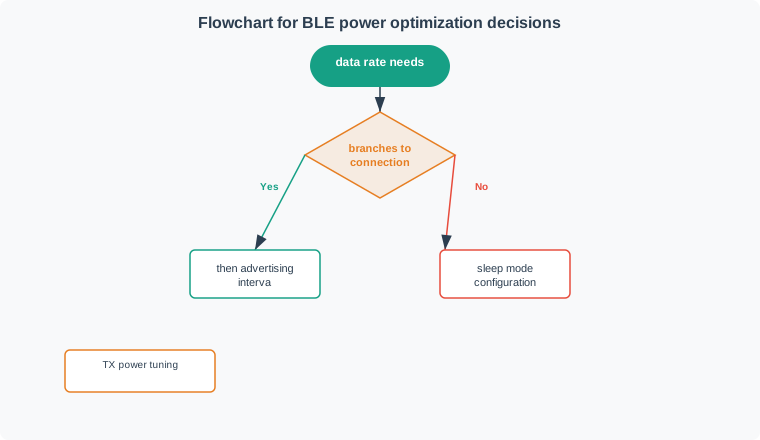
17.8 BLE Power Optimization Decision Flow
When building battery-powered BLE devices, power optimization is critical:
17.9 Visual Reference Gallery
Visual: BLE Module Architecture
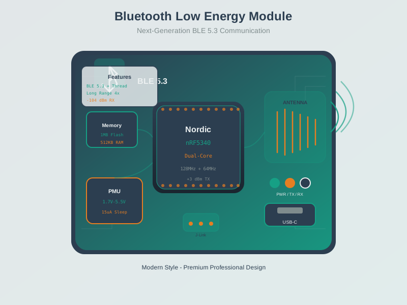
BLE modules integrate radio, processor, and antenna for easy integration into IoT device designs.
Visual: BLE GATT Profile Implementation
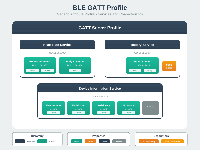
GATT implementation requires defining services and characteristics with appropriate properties for your application’s data model.
Visual: BLE Connection Flow
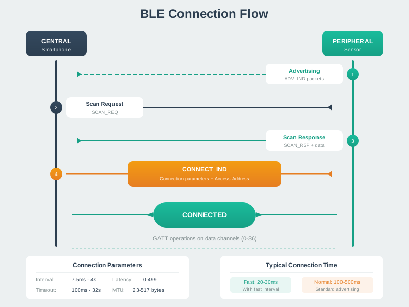
Understanding the connection flow helps optimize connection latency and power consumption in BLE applications.
Visual: BLE Stack Architecture
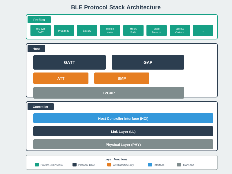
The BLE stack provides standardized interfaces for application developers to build interoperable devices.
Visual: Bluetooth Serial Port Profile
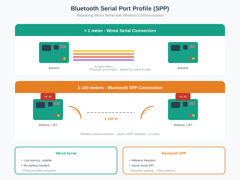
SPP enables legacy serial applications to communicate wirelessly, useful for debugging and configuration interfaces.
17.10 Knowledge Check
17.10.1 Knowledge Check: BLE Scanning and Filtering
17.10.2 Knowledge Check: GATT Service Exploration
17.10.3 Knowledge Check: BLE Proximity Detection
17.11 Deployment Pattern: BLE Proximity System for Retail Analytics
Retail analytics systems often use BLE proximity detection to estimate customer dwell time and foot-traffic patterns. A typical design places Python gateways on small Linux computers near entrances and key departments, then classifies nearby beacon traffic into immediate, near, and far zones.
System Specifications:
- Scan interval:
2 seconds, balancing detection speed against gateway CPU load. - RSSI threshold:
-75 dBm, filtering devices beyond the useful local radius. - EMA alpha:
0.2, prioritizing stability over responsiveness for dwell-time estimates. - Zone boundaries:
-55 dBmand-70 dBm, mapping readings to immediate, near, and far zones. - Minimum samples:
3, requiring consecutive readings before assigning a zone. - Gateway density:
4to6gateways for a medium retail floor, adjusted after site survey testing.
Why EMA Alpha = 0.2 (Not 0.3)?
The standard alpha of 0.3 works well for single-device tracking, but in a crowded retail environment with 50-200 simultaneous BLE advertisers, lower alpha reduces false zone transitions caused by body shadowing. A customer stepping behind a display rack causes a sudden 10-15 dBm drop. With alpha 0.3, the smoothed RSSI reacts in 2 readings (4 seconds), potentially triggering a false “far” classification. With alpha 0.2, it takes 4 readings (8 seconds) – long enough for the customer to move again, preventing a spurious zone change.
Battery Impact on Beacons:
Assume a BLE beacon with a 1000 mAh battery advertising at 1 Hz:
- Advertising current per event:
8 mA. - Event duration, including radio ramp-up:
3 ms. - Events per day at
1 Hz:86,400. - Daily energy at
1 Hz:8 mA x 0.003 s x 86,400 = 2,073.6 mA-s, and dividing by3,600converts to0.576 mAh/day. - Estimated battery life at
1 Hz:1000 mAh / 0.576 mAh = 1,736 daysfrom advertising alone – sleep current and sensor reads shorten this in practice. - Estimated battery life at
10 Hz: about174 days, because daily energy rises to5.76 mAh/day.
This is why many deployments prefer 1 Hz advertising with gateway-side EMA smoothing. Raising the advertising rate by 10x can make detection feel faster, but it also turns a maintenance interval measured in years into one measured in months.
Checkpoint: Deployment Trade-Offs
You now know:
- The retail pattern combines a
2 secondsscan interval,-75 dBmfilter, alpha0.2,-55 dBmand-70 dBmzone boundaries, and3consecutive samples before assigning a zone. - For a
1000 mAhbeacon advertising at1 Hz, the chapter’s arithmetic gives0.576 mAh/dayand about1,736 daysfrom advertising alone. - Raising the rate to
10 Hzimproves responsiveness but cuts the advertising-only estimate to about174 days, so gateway-side smoothing is often the better maintenance choice.
At this point the script has enough design context to be reviewed. The remaining sections test whether the same choices survive quizzes, runtime limits, disconnections, and common implementation mistakes.
Concept Relationships:
- RSSI filtering and zone-based detection: Threshold filtering reduces noise from distant devices before zone classification runs.
- EMA smoothing and proximity detection: Exponential moving average stabilizes noisy RSSI readings so zones do not flicker.
- GATT explorer and service discovery: Enumerating UUIDs maps device capabilities before data access.
- Beacon protocols and indoor positioning: iBeacon and Eddystone formats provide repeatable advertisement structures for location services.
- bleak and cross-platform support: One async Python API can target Windows, macOS, and Linux backends.
17.12 See Also
- BLE Hands-On Labs - Complete project implementations with heart rate monitors and positioning
- BLE Code Examples - Basic Python scanner patterns and GATT concepts
- Bluetooth Security - Understanding secure device pairing
- Bluetooth Applications - Real-world BLE deployment case studies
17.13 Practice Activities
17.14 Start With the Story
A laptop running Python can turn BLE from a black box into a repeatable inspection tool. Scans, filters, UUIDs, GATT reads, notifications, RSSI samples, and exceptions become evidence a team can rerun.
Use this chapter to make automation serve the design review. Write the smallest Bleak script that observes the claim, log the result, and connect the script output back to the device behavior it is meant to prove.
17.15 Deep Dive: Bleak Role Boundaries and Runtime Limits
Bleak is a Central/client API. A modern BLE controller can time-slice more than one role, but Bleak exposes the Python host as the scanner, initiator, and GATT client. If the same product also needs a phone to discover the Python host or read a characteristic served by it, that Peripheral/server role needs firmware support or a platform-specific peripheral stack.
The scaling constraint is usually scheduling, not Python byte throughput. A gateway subscribed to 12 peripherals sending one 20 byte notification each second handles only about 240 payload bytes per second, but the controller still schedules every connection event and the OS backend still delivers every callback. Keep notification callbacks short: decode the packet, attach a timestamp, enqueue the record, and return. File writes, MQTT publishes, and database retries belong outside the BLE callback path.
ATT framing also changes what a successful trace proves. With the default ATT MTU, a notification commonly carries up to 20 application bytes after overhead. A 38 byte sensor report needs MTU negotiation or application-level chunking with an order field and a missing-chunk timeout. Otherwise a clean connection log can still hide truncated data.
| Runtime concern | Evidence to keep in the review log |
|---|---|
| Role fit | Python host is named as Central/GATT client; firmware tag is named as Peripheral/GATT server. |
| Callback pressure | Notification handler returns quickly and pushes timestamped records into an async queue. |
| Payload size | MTU or chunking plan covers records larger than one notification payload. |
| Disconnection policy | Disconnect callback, bounded backoff, reconnect/rescan policy, and stale-sensor interval are recorded. |
Disconnects are normal events. For a 2 second sample period, marking a sensor stale after 10 seconds means five missed samples; that explicit timing assumption is easier for the rest of the IoT pipeline to reason about than a generic “retry forever” loop.
17.16 Summary
This chapter covered production Python BLE implementations:
- Scanner with Filtering: RSSI thresholds and name pattern matching for targeted device discovery
- GATT Explorer: Enumerating services and characteristics on connected devices
- Beacon Management: Parsing iBeacon and Eddystone advertisement formats
- Proximity Detection: Zone-based presence detection with exponential smoothing
- Power Optimization: Decision framework for connection intervals and advertising parameters
Worked Example: RSSI-to-Distance Calculation and Zone Classification
Scenario: A Python BLE proximity system measures RSSI from iBeacons to determine customer location in a retail store. Calculate distance and classify into zones.
Given beacon parameters:
- TX Power at 1 meter: -59 dBm (calibrated value from manufacturer)
- Path loss exponent (n): 2.5 (typical retail environment with shelves)
- RSSI measurements (5-sample moving average): [-68, -72, -65, -70, -66] dBm
Step 1: Calculate smoothed RSSI using exponential moving average
alpha = 0.3  # EMA smoothing factor
rssi_samples = [-68, -72, -65, -70, -66]

smoothed = rssi_samples[0]  # Initialize with first sample
for rssi in rssi_samples[1:]:
    smoothed = alpha * rssi + (1 - alpha) * smoothed
    print(f"RSSI {rssi} → Smoothed {smoothed:.1f}")
Output:
RSSI -72 → Smoothed -69.2
RSSI -65 → Smoothed -67.9
RSSI -70 → Smoothed -68.6
RSSI -66 → Smoothed -67.8
Smoothed RSSI: -67.8 dBm
Step 2: Calculate distance using log-distance path loss model
Formula: d = 10 ^ ((TxPower - RSSI) / (10 * n))
Where: - TxPower = -59 dBm (calibrated at 1 meter) - RSSI = -67.8 dBm (smoothed) - n = 2.5 (path loss exponent)
import math

tx_power = -59
rssi = -67.8
n = 2.5

distance = 10 ** ((tx_power - rssi) / (10 * n))
print(f"Distance: {distance:.2f} meters")
Calculation:
- (−59 − (−67.8)) / (10 × 2.5) = 8.8 / 25 = 0.352
- 10^0.352 = 2.25 meters
Step 3: Classify into proximity zones
def classify_zone(rssi):
    if rssi > -55:
        return "immediate", "< 0.5m"
    elif rssi > -70:
        return "near", "0.5 - 3m"
    else:
        return "far", "> 3m"

zone, range_desc = classify_zone(-67.8)
print(f"Zone: {zone} ({range_desc})")
Result: Zone = “near” (0.5 - 3m), calculated distance = 2.25m.
Step 4: Account for uncertainty
Representative RSSI variance in retail-like environments: - Standard deviation: +/-6 dBm - Distance range at 2.25m, from the log-distance model with n = 2.5 (not a symmetric +/-meters band, because distance is an exponential, not linear, function of RSSI): a +6 dBm weaker reading scales distance by 10^(6/25) = 1.74x, to about 3.91m; a -6 dBm stronger reading scales it by 10^(-6/25) = 0.575x, to about 1.29m
Conclusion: The beacon is roughly 1.3 to 3.9 meters away (point estimate 2.25m), classified as “near” zone from its RSSI threshold regardless of that spread. This asymmetric, meter-scale uncertainty is exactly why zone-based classification – not a precise distance figure – is the reliable output here. For applications requiring sub-meter accuracy, compare BLE RSSI with UWB positioning instead.
Decision Framework: Choosing BLE Python Library (bleak vs alternatives)
For new BLE GATT work, start with bleak unless you have a specific platform or Classic Bluetooth requirement.
Library fit:
- bleak: Cross-platform BLE GATT scanning, connection, read, write, notify, and indicate workflows with native
asyncio. - bluepy: Linux-focused synchronous BLE code. Treat it mainly as a legacy-code dependency unless your deployment already standardizes on it.
- pybluez: Useful for Classic Bluetooth workflows such as Serial Port Profile, but not a replacement for a BLE GATT library.
- pygatt: Can support simple BLE workflows, but is usually less flexible for cross-platform async gateway code.
Decision path:
- Need cross-platform BLE scanning or GATT access: choose bleak.
- Need an async gateway or UI-backed application: choose bleak and keep BLE work off blocking callbacks.
- Maintaining an existing Linux-only script: keep the existing library only if the support burden is acceptable.
- Need Classic Bluetooth rather than BLE: use a Classic Bluetooth library or platform API instead of a BLE GATT library.
- Before production use: check the project’s current release history, supported Python versions, and operating-system backend notes.
Minimal bleak scanner:
import asyncio
from bleak import BleakScanner

async def scan():
    devices = await BleakScanner.discover(timeout=10)
    for dev in devices:
        print(dev.address, dev.rssi)

asyncio.run(scan())
Common Mistake: Not Handling BLE Disconnections in Long-Running Scripts
The error: A Python script using bleak connects to a BLE temperature sensor, reads data in a loop, but doesn’t handle disconnections. After 15 minutes, the script crashes when the sensor goes to sleep.
What happens:
import asyncio
from bleak import BleakClient

async def monitor_temperature():
    address = "A4:CF:12:34:56:78"
    async with BleakClient(address) as client:
        while True:
            # Read temperature characteristic
            temp_bytes = await client.read_gatt_char("0x2A6E")
            temp = int.from_bytes(temp_bytes, 'little') / 100.0
            print(f"Temperature: {temp}°C")
            await asyncio.sleep(60)  # Read every minute

asyncio.run(monitor_temperature())
Failure scenario:
- Script connects successfully
- Reads temperature for 15 minutes
- Sensor enters low-power mode (connection supervision timeout)
- Line
temp_bytes = await client.read_gatt_char()raisesBleakError: Not connected - Script crashes with unhandled exception
The fix (production-grade with reconnection):
import asyncio
from bleak import BleakClient
from bleak.exc import BleakError

async def monitor_temperature():
    address = "A4:CF:12:34:56:78"

    while True:  # Outer loop for reconnection
        try:
            async with BleakClient(address, timeout=20) as client:
                print(f"Connected to {address}")

                while True:  # Inner loop for reading
                    try:
                        temp_bytes = await client.read_gatt_char("0x2A6E")
                        temp = int.from_bytes(temp_bytes, 'little') / 100.0
                        print(f"Temperature: {temp}°C")
                        await asyncio.sleep(60)

                    except BleakError as e:
                        print(f"Read error: {e}, will reconnect")
                        break  # Exit inner loop to trigger reconnect

        except BleakError as e:
            print(f"Connection failed: {e}, retrying in 5s")
            await asyncio.sleep(5)
        except KeyboardInterrupt:
            print("Stopped by user")
            break

asyncio.run(monitor_temperature())
What this adds:
- Outer while loop: Retries connection if it fails initially or drops
- Inner try/except: Catches read errors, triggers reconnection
- Timeout parameter: Prevents hanging on slow connections
- KeyboardInterrupt: Allows graceful shutdown with Ctrl+C
- Backoff delay: 5-second wait between reconnect attempts (prevents busy loop)
Production enhancement (exponential backoff):
retry_delay = 5
max_delay = 60

while True:
    try:
        async with BleakClient(address) as client:
            retry_delay = 5  # Reset on successful connect
            # ... reading loop ...
    except BleakError:
        print(f"Retrying in {retry_delay}s")
        await asyncio.sleep(retry_delay)
        retry_delay = min(retry_delay * 2, max_delay)  # Exponential backoff
Measured reliability improvement:
A data logging project ran for 30 days: - Without reconnection logic: 12 crashes (script stopped after first disconnect) - With reconnection: 0 crashes, 99.2% uptime (0.8% was unavoidable sensor reboot time)
Rule of thumb: All production BLE scripts need reconnection logic. BLE is wireless and inherently unreliable—disconnections are normal, not exceptions.
Common Pitfalls
1. Not Awaiting bleak Coroutines
bleak is fully asynchronous; calling client.read_gatt_char(uuid) without await returns a coroutine object, not the data. Comparing a coroutine object to expected values always produces False. Every bleak operation must use await: data = await client.read_gatt_char(uuid). If you see <coroutine object…> in print output, you forgot await.
2. Scanning by Name in Noisy Environments
Using BleakScanner.find_device_by_name(“MySensor”) in an environment with many BLE devices is slow and unreliable — it scans until timeout if the device is temporarily out of range. Use BleakScanner.find_device_by_filter() with a service UUID filter instead: scanner.find_device_by_filter(lambda d, adv: SERVICE_UUID in adv.service_uuids). This is more specific and faster than name-matching.
3. Blocking the asyncio Event Loop in Notification Callbacks
bleak notification callbacks run in the asyncio event loop thread. Calling blocking operations (time.sleep(), file.write() with large payloads, synchronous DB writes) inside callbacks freezes BLE processing and causes missed notifications. Use asyncio.create_task() to schedule data processing, or write to an asyncio.Queue() and process in a separate coroutine.
4. Assuming Consistent Service/Characteristic Handle Order
GATT service discovery order is not guaranteed to be consistent across firmware versions or device resets. Caching the handle integer directly (e.g., handle = 0x000E) and using it in subsequent sessions is fragile. Always use UUID-based access: client.read_gatt_char(“0000xxxx-0000-1000-8000-00805f9b34fb”). Let bleak resolve the handle internally on each connection.
17.17 What’s Next
Prioritize these follow-up chapters based on the implementation problem you are solving:
- BLE code examples: bt-impl-code-examples.html for foundational scanner, GATT client, and notification patterns.
- BLE hands-on labs: bt-impl-labs.html for complete projects that combine scanning, services, proximity, and mesh concepts.
- Bluetooth security: bluetooth-security.html for pairing, bonding, encryption, and threat modeling before production deployment.
- BLE pairing methods: bt-security-pairing-methods.html for authenticated subscriptions and bonded devices.
- BLE encryption keys: bt-security-encryption-keys.html for LTK, IRK, CSRK, and re-connection behavior.
- Bluetooth applications: bluetooth-applications.html for deployment scenarios that use BLE gateways, beacons, and wearables.
- UWB positioning systems: ../rfid-nfc-uwb/uwb-positioning-systems.html when BLE RSSI zones are not accurate enough.
- Bluetooth fundamentals and architecture: bluetooth-fundamentals-and-architecture.html to connect Python API behavior back to GAP, GATT, ATT, and link-layer concepts.
17.18 Key Takeaway
Python BLE code must handle asynchronous discovery, connection loss, notification callbacks, and platform differences. Keep scripts event-driven and defensive rather than assuming every peripheral behaves like a stable serial port.