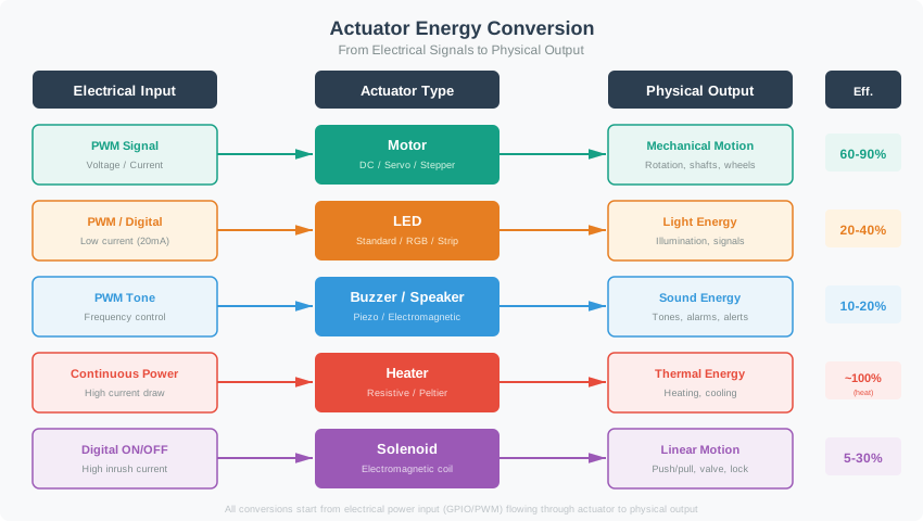
In the lab, the story starts before the first jumper wire. Decide what motion, light, sound, or switching result you expect; predict the current path and safe state; then run the smallest test that proves the actuator did what you asked.
Use the browser labs as rehearsal for the physical bench. A good lab record connects command, driver, load, observation, and fault handling so a working demo becomes repeatable evidence rather than a lucky spin or beep.
In 60 Seconds
These hands-on labs guide you through building complete actuator control systems, from DC motor speed ramping and servo-based robotic grippers to multi-actuator systems and PID feedback control. Each lab uses browser-based interaction first, then ESP32 code, so students can reason about actuator behavior before touching hardware.
Phoebe’s Field Notes: Why “0.25 x 255 = 64” Is Not The Exact Speed
Phoebe’s Why
Lab 1’s ledcSetup(pwmChannel, pwmFreq, pwmResolution) line is doing two separate jobs, and this chapter’s own troubleshooting note (“students should not assume those values mean exact speed”) is really a statement about the second one. The 8-bit pwmResolution turns a continuous 0-100% command into one of 256 discrete duty-cycle codes – the same rounding-to-a-code physics that limits any ADC, just running in reverse to make an analog-ish output instead of reading one in. The 5 kHz pwmFreq is a different question: it has to switch fast enough that the motor’s own winding inductance, not the driver, is what smooths the chopped voltage into something close to steady current. Get the resolution wrong and every commanded speed is off by a fixed, computable amount; get the switching frequency wrong relative to the motor’s electrical time constant and the winding never averages the pulses at all.
The Derivation
Quantization step and RMS noise for an \(N\)-bit duty-cycle code driving supply voltage \(V_{supply}\):
The chopped PWM only averages into a steady current if the switching frequency clears that corner with the same kind of margin a sampled signal needs above Nyquist:
\[f_{PWM} \gg 2f_c\]
Worked Numbers: This Chapter’s 8-Bit, 5 kHz, 9 V Channel
Voltage LSB on the 9 V motor supply: \(q=9/256=0.0352\) V \(=35.2\) mV per code step – so “25% PWM” landing on code 64 instead of the algebraic \(0.25\times255=63.75\) is exactly the kind of rounding this chapter’s own examples (64, 191, 51 for 25%, 75%, 20%) already show without naming it.
Quantizer SNR at 8 bits: \(\mathrm{SNR}=6.02\times8+1.76=49.9\) dB – the physical reason a measured “supply drops from 9.0 V to 7.8 V at startup” (this chapter’s own flyback/wiring-stress check) has to be read off the multimeter, not inferred from the PWM code.
Switching-versus-winding check with a catalog-typical small brushed DC motor (\(R=6\ \Omega\), \(L=1.5\) mH): \(\tau=L/R=0.250\) ms, \(f_c=1/(2\pi\tau)=637\) Hz. This chapter’s own 5 kHz PWM sits at \(5{,}000/637=7.85\times\) the corner frequency – about \(3.93\times\) the \(2f_c\) margin a clean average needs – which is why the L298N lab can treat “PWM speed” as smooth motor voltage instead of an audible or jerky chop.
Learning Objectives
After completing these labs, you will be able to:
Construct complete actuator control systems from scratch using ESP32 and motor drivers
Integrate multiple actuator types (DC motors, servos, buzzers, LEDs) in a single project
Implement coordinated multi-axis motion control with synchronized timing
Validate actuator designs with browser-based simulations before hardware deployment
Diagnose and resolve common actuator wiring, power, and control problems
For Beginners: Actuator Labs
These labs are like cooking recipes for electronics – they walk you through building real circuits step by step, from connecting wires on a breadboard to writing code that makes motors spin and buzzers beep. Start with the built-in browser labs on this page, then move to real hardware or an external circuit simulator when you are ready.
Chapter Roadmap
Use these labs as a controlled bench sequence:
First prove the DC motor path: GPIO26/GPIO27 for direction, GPIO14 for PWM, and the external 9 V motor supply.
Then build the three-servo gripper with a separate 5 V 2 A supply, common ground, and gradual interpolation.
Next combine fan, vent, LED, and buzzer outputs in the browser lab before wiring the challenges.
Finally close the loop with PID evidence, troubleshooting checks, and the quizzes.
12.2 Lab 1: DC Motor Control with L298N
Objective: Control a DC motor using the L298N H-bridge driver with smooth acceleration and deceleration.
Run it: Warm up for these challenges with the actuator-selection game below, which mirrors their Beginner, Intermediate, and Advanced structure. Each scenario asks you to choose the actuator that best satisfies the engineering constraints – matching motor, servo, PWM, and signalling choices to a stated requirement – so you commit to a control approach before you wire it. Clear the Beginner tier to lock in the traffic-light and speed mappings, then push into Intermediate and Advanced to rehearse the temperature-responsive control logic Challenge 3 asks you to build.
Challenge 1: Traffic Light Controller (Beginner)
Create a traffic light using the RGB LED:
Red for 5 seconds
Yellow for 2 seconds
Green for 5 seconds
Yellow for 2 seconds
Repeat
Add a buzzer beep when changing to green (pedestrian signal).
Challenge 2: Speed-Responsive Motor (Intermediate)
Use a potentiometer to control:
DC motor speed (0-100%)
LED brightness (proportional to speed)
Buzzer pitch (higher = faster)
Challenge 3: Smart Fan Controller (Advanced)
Implement a temperature-responsive fan:
Read temperature from sensor (or simulate with potentiometer)
Below 20C: LED blue, motor off
20-25C: LED green, motor 50%
25-30C: LED yellow, motor 75%
Above 30C: LED red, motor 100%, alarm buzzer
A Raspberry Pi version of the same lab can use a DHT22 temperature and humidity sensor, a 4.7 k ohm pull-up on the data line, and a relay module to switch a small fan. The lab evidence should record the DHT power, data, and ground pins; the GPIO pin that drives the relay input; whether the relay uses the normally-open or normally-closed contact; and the exact threshold rule, such as fan on above 30 C and off again only after a deliberate deadband. The important lesson is not the library name or board brand. It is the sensor-to-actuator loop: read the environment, decide locally, drive a separately powered load through a safe interface, and prove the fan state changed when the threshold was crossed.
Checkpoint: Multi-Actuator Rules
You now know:
Browser rules map temperature at 24 C, 28 C, and 35 C; emergency mode forces fan 100 percent and vent 90 degrees.
The smart fan bands are explicit: below 20 C off, 20-25 C at 50 percent, 25-30 C at 75 percent, and above 30 C at 100 percent with alarm.
The Raspberry Pi evidence chain is DHT22 reading, 4.7 k ohm pull-up, relay GPIO, contact choice, and deliberate deadband.
Lab 4 adds encoder feedback and PID tuning so the motor can correct speed error instead of merely receiving a duty cycle.
12.5 Lab 4: Advanced PID Control
This lab implements PID feedback control for precise motor speed regulation.
12.5.1 Learning Objectives
Apply PID controller theory to tune proportional, integral, and derivative gains
Implement encoder feedback for closed-loop speed control
Analyze control loop behavior and diagnose oscillation issues using Serial Monitor
12.5.2 Key Concepts
Proportional Term (P):
Output = Kp x Error
Responds to current error. Higher Kp = faster response but may overshoot.
Integral Term (I):
Output = Ki x Integral(Error)
Eliminates steady-state error. Higher Ki = faster correction but may oscillate.
Derivative Term (D):
Output = Kd x Derivative(Error)
Dampens oscillations. Higher Kd = more stability but sensitive to noise.
12.5.3 Tuning Guide
Start with Kp = 1, Ki = 0, Kd = 0
Increase Kp until system oscillates
Reduce Kp by 50%
Add Ki to eliminate steady-state error
Add Kd if oscillations occur
Putting Numbers to It
PID controller proportional term determines how aggressively the system responds to speed error in motor control.
If current PWM is 128 (50% duty), add 25 to reach 153 (60% duty), increasing motor speed. Higher \(K_p\) values respond faster but may overshoot and oscillate — typical starting values are 0.1-1.0 for motor speed control applications.
Start with Kp = 1, Ki = 0, and Kd = 0, then increase Kp until oscillation appears and reduce it by 50 percent.
The worked example uses 300 RPM target, 250 RPM measured, 50 RPM error, and Kp = 0.5 to add 25 PWM counts.
The calculator clamps the command between 0 and 255, so the record shows both the calculation and the duty-cycle limit.
After that, separate wiring, power, thermal, and feedback faults before changing gains again.
12.6 Troubleshooting Guide
Problem
Possible Cause
Solution
Motor doesn’t spin
Wrong wiring
Check IN1, IN2, and EN connections
Motor only spins one direction
Direction pins swapped
Swap IN1 and IN2
Servo jitters
Insufficient power
Use external 5V supply
Stepper skips steps
Acceleration too fast
Reduce max speed, increase acceleration time
Driver overheats
Current too high
Add heatsink, reduce motor current
Random resets
Missing flyback diode
Add diode across inductive loads
Coordinated Servo Speed Sizing
Problem: A 2-DOF robotic arm must move from position A (base=45°, arm=45°) to position B (base=135°, arm=90°) in exactly 2 seconds. Both servos must arrive simultaneously to prevent jerky motion. Calculate the required speeds for each servo.
Given Servo Specifications (SG90):
Speed rating: 0.1 seconds / 60 degrees at 5V
This means: 60° rotation takes 0.1 seconds
Or: 600 degrees per second maximum speed
Step 1: Calculate Angular Distance for Each Servo
Base servo:
Start: 45°
End: 135°
Distance: 135° - 45° = 90° rotation
Arm servo:
Start: 45°
End: 90°
Distance: 90° - 45° = 45° rotation
Step 2: Calculate Required Angular Velocity
Both servos must complete in 2 seconds:
Base servo speed: 90° ÷ 2 seconds = 45°/second
Arm servo speed: 45° ÷ 2 seconds = 22.5°/second
Step 3: Verify Speed is Within Servo Capability
SG90 maximum speed: 600°/second
Both required speeds (45°/s and 22.5°/s) are well below the 600°/s maximum, so this motion is achievable.
moveToPosition(135,90,2000);// Base to 135°, Arm to 90°, in 2000ms
Step 5: Calculate Actual Step Increments
With 2000ms duration and 20ms steps: - Total steps: 2000 ÷ 20 = 100 steps
Base servo:
90° total ÷ 100 steps = 0.9° per step
Arm servo:
45° total ÷ 100 steps = 0.45° per step
Step 6: Verify Servo Can Achieve Step Resolution
SG90 servos typically have: - Control resolution: 1° (can position to nearest degree) - Our increments: 0.9° and 0.45° per step
Since we’re commanding sub-degree increments, the servo’s internal control will round to nearest degree, creating very smooth motion with minimal visible stepping.
Real-World Complications:
Issue 1: Servo Speed Variance
Datasheet says 0.1s/60° but real servos vary by ±20%
Solution: Measure actual servo speed, adjust timing
Issue 2: Different Servo Models
Base servo (metal gear MG996R): 0.17s/60° (slower)
Arm servo (SG90): 0.1s/60°
They’ll arrive at different times!
Solution for Mixed Servos:
// Calculate minimum time for each servo (distance * seconds_per_degree)float baseTime =90.0*(0.17/60.0);// = 0.255 seconds minimumfloat armTime =45.0*(0.10/60.0);// = 0.075 seconds minimum// Convert to milliseconds and use the longer time as the floorint minDurationMs = max((int)(baseTime *1000),(int)(armTime *1000));// 255 msint duration = max(minDurationMs,2000);// Use 2000 ms for smooth motion
Key Insight: Coordinated multi-axis motion requires: 1. Calculate each axis’s travel distance 2. Normalize all axes to same total time 3. Break motion into small steps (20ms intervals for servos) 4. Account for different servo speeds if mixing models 5. Use linear interpolation for smooth, synchronized arrival
Extension: Non-Linear Motion (Ease-In/Ease-Out)
For more natural motion, use easing functions:
float easeInOutCubic(float t){return t <0.5?4* t * t * t :1- pow(-2* t +2,3)/2;}// In loop:float progress = easeInOutCubic((float)i /(float)steps);
This starts slow, speeds up in middle, slows at end—much more human-like than linear motion.
12.7 Knowledge Check
Question: PID Proportional Gain
12.8 Deep Dive: Driver Power Paths and Common Ground
The first hands-on lesson is a prohibition: never wire a motor, solenoid, or relay coil straight to a microcontroller pin. A GPIO can only source or sink a few tens of milliamps, while even a small motor wants hundreds of milliamps to amps. The pin’s real job is to carry a control signal to a driver that handles real current from a separate supply.
Figure 12.1: Use lab notes to record both sides of the actuator interface: the command signal that describes the action and the powered load that converts electrical energy into a physical output.
In the DC motor lab, GPIO14 sends PWM to the L298N enable input while GPIO26 and GPIO27 choose H-bridge direction. The motor supply is the external 9 V rail, not the ESP32 pin. If the motor draws 0.35 A while spinning freely, the running motor power is about 9 x 0.35 = 3.15 W. If it draws 1.4 A at startup or during a brief stall, the driver and supply must tolerate that surge even though the GPIO signal is still only logic-level.
The same rule applies to servos. A signal pulse from the controller may be only a timing command, but the servo’s power wires carry real actuator current. Three small servos that each draw 600 mA when loaded can demand 3 x 0.6 = 1.8 A. That is far beyond the safe budget of a USB-powered board. The lab should separate signal wiring from load power and then prove that all grounds share a reference.
Interface
Good for
Lab evidence to record
Low-side MOSFET or transistor
One-direction on/off loads such as motors, solenoids, or relay coils
Logic threshold, flyback path, current draw, timeout behavior
H-bridge driver IC
Reversible motors with PWM speed
Forward/reverse/coast/stop behavior, driver temperature, supply sag
Turn each lab into a measurement record. At 25% PWM on an 8-bit channel, the command value is about 0.25 x 255 = 64. At 75%, it is about 0.75 x 255 = 191. Students should not assume those values mean exact speed; they should measure current, observe shaft behavior, and record whether the supply voltage dips when the motor starts. If the measured supply drops from 9.0 V to 7.8 V at startup, that is evidence of source or wiring stress, not a software bug.
For a one-direction solenoid or relay coil, the checklist is shorter but stricter: driver transistor, coil supply, common ground, flyback diode, and timeout. If a 12 V solenoid draws 450 mA, the coil dissipates 12 x 0.45 = 5.4 W while energized. A short pulse may be safe; a forgotten always-on output can overheat the coil. For reversible motors, verify direction at low duty before speed. Start at 20% PWM, about 0.20 x 255 = 51 on an 8-bit channel, then confirm forward, reverse, coast, and stop behavior before increasing load.
Motors are electrically noisy and often want a higher voltage than the logic, so power them from a separate supply rather than the microcontroller’s regulator. But the two supplies must share a common ground. A logic signal is only meaningful as a voltage relative to a reference, so the driver’s control input needs the same ground as the microcontroller; without it, “high” and “low” are undefined and the driver behaves erratically or not at all.
Grounding is not just a wiring diagram convention; it changes the voltage the driver sees. If the motor return carries a 1.5 A startup surge through 0.2 ohm of shared breadboard wiring, that path can move by 1.5 x 0.2 = 0.3 V. A logic input that should be a clean 3.3 V high may become noisy relative to the driver, and the ESP32 may reset if the same sag reaches its supply. Star-style grounding and short, thick motor-return paths reduce that shared impedance.
Decoupling has the same practical role. A bulk capacitor near the driver supplies brief current while the battery or bench supply catches up; a small ceramic capacitor handles faster switching edges. A lab note such as “motor startup dips from 5.0 V to 4.4 V without bulk capacitance, but only to 4.8 V with it” is stronger evidence than “it seems stable.” The safe topology is logic power for logic, motor power for the load, one deliberate ground reference, and a driver between them.
12.9 Summary
Actuator labs expose the practical behavior that datasheets and theory can hide: startup current, wiring looseness, mechanical direction, timing jitter, and the need for gradual motion profiles. The safest lab flow is simulate, measure current, test at low power, then increase load only after direction and protection are verified.
Key Takeaway
Hands-on labs are essential for understanding actuator behavior that theory alone cannot convey, including power supply limitations, real-world timing constraints, and the importance of smooth acceleration profiles. Always prototype with browser-based simulations or a safe circuit simulator before moving to physical hardware, and remember that proper power supply design is as important as the control code itself.
For Kids: Meet the Actuator Crew!
“Lab day! Lab day!” cheered Lila the LED, blinking excitedly. The Actuator Crew had set up a mini workshop.
“Okay team,” said Max the Microcontroller, “today we’re building a robot arm! Servo Sam, you’re in charge of the joints.”
Servo Sam flexed his gears. “Base rotation – check! Arm lift – check! Gripper – check! I can move to any angle you tell me, Max!”
“But wait,” Bella the Battery said worriedly. “Three servos? That’s a lot of power! Don’t you dare try to power them all through Max – he’ll overheat!”
“Good thinking, Bella!” said Max. “We need a big external power supply for the servos. I just send them tiny signal messages telling them where to go. The heavy lifting power comes from elsewhere.”
Sammy the Sensor watched as the arm picked up a small block. “I can see the arm is at 45 degrees… now closing the gripper… now lifting! It’s working!”
“The secret,” Max explained, “is smooth movements. If I tell all the servos to jump to new positions instantly, the arm jerks around and might knock things over. Instead, I move them gradually – a little bit at a time – like doing a slow-motion dance!”
“Building is the best way to learn!” Lila flashed in agreement.
The appropriate transistor, MOSFET, or H-bridge IC depends critically on the actuator’s actual current draw. Without measuring current with a multimeter in series, you might select a driver rated for 500 mA for a motor that draws 800 mA under load, causing driver overheating or failure during the lab. Measure current in your specific circuit before finalizing component selection.
2. Skipping Motor Direction Verification Before Speed Control
When implementing H-bridge DC motor control, verify direction behavior with low PWM duty cycle (20-30%) before incrementing to full speed. Running a motor at full speed in the wrong direction can mechanically damage the mechanism being driven. Always confirm correct rotation direction at low speed first.
3. Secure Lab Motor Wiring
Motor vibration and cable tension cause breadboard connections to loosen during operation, producing intermittent faults difficult to diagnose. Use wire colors consistently (red for power, black for ground, yellow/green for signals), press connectors firmly into breadboard holes, and consider twist-tying cable bundles to reduce mechanical stress on connections.
4. Not Implementing Ramp-Up in Motor Control Lab Firmware
Starting a motor at 100% PWM immediately causes maximum inrush current, which can trigger power supply protection, cause microcontroller brownout resets, or mechanically stress the driven mechanism. In lab firmware, always ramp PWM duty cycle from 0 to target over 500 ms - 2 seconds to control startup current and reduce mechanical shock.
12.11 What’s Next?
Now that you have completed the hands-on labs, deepen your understanding with the theory chapters or test your knowledge with the assessment.

 Checkpoint: H-Bridge Bench Pass