2 Media Compression Mechanics: Audio, Image, and Video
2.1 Overview: Remove What the Receiver Cannot Use
Data Encoding and Codecs already establishes the decision layer: a media codec applies decomposition, quantization, and entropy coding, and a product team chooses among codecs by fidelity, latency, compute, compatibility, and replay needs. This chapter does not repeat that taxonomy. It opens the mechanism underneath it: how perception makes some audio error irrelevant, how an image block becomes spatial-frequency coefficients, and how a video encoder predicts motion before coding what remains.
The useful distinction is between two kinds of savings:
- Statistical redundancy means the source contains values that can be represented more compactly without changing the reconstruction.
- Perceptual irrelevancy means a changed reconstruction can still be indistinguishable, or acceptably close, for the intended listener or viewer.
Lossy media coding uses both. The risk is also in that sentence: “irrelevant” is never universal. It depends on the signal, the listener or viewing task, the playback path, and the encoder settings.
2.1.1 Psychoacoustic Masking Is a Moving Threshold
The threshold in quiet is the minimum sound-pressure level a typical listener can detect at each frequency in a quiet environment. It is not flat: human hearing is most sensitive through part of the mid-frequency range and less sensitive at very low and very high frequencies. A strong tone or narrow band of energy raises that detection threshold around itself. Energy below the raised masking threshold is present physically but is less likely to be heard.
That is the mechanism a perceptual audio encoder exploits. It estimates energy across time and frequency, predicts which quantization noise would fall below the local masking threshold, and spends fewer bits where the resulting error is least audible. The encoder is not deleting “high frequencies” as a single rule. It is allocating error against a threshold that changes with the signal.
Quiet threshold
The baseline detectability curve varies with frequency even when no masker is present.
Masker
A strong component raises the nearby threshold; its effect spreads unevenly across frequency and time.
Noise allocation
Quantization error is shaped toward regions where the model predicts it will remain below that threshold.
The source lecture makes this audible with the 1990 Brandenburg and Johnston “Miracle 13dB” demonstration. Its four listening conditions are:
A. Original
The reference signal without added noise.
B. White noise
The original plus spectrally broad noise at -13 dB relative to the signal; the noise is obvious.
C. Shaped noise
The same nominal noise-to-signal relationship, but shaped against the signal's masking threshold; it can be difficult to hear.
D. Difference
The removed or added component heard on its own, proving that substantial energy can be perceptually hidden.
This page does not counterfeit the listening test. The source slide points to audio examples, but the estate does not contain licensed A/B/C/D assets for this demonstration. The registry-matched workbench below can generate tone-plus-noise and expose RMS and spectrum; it is a frequency-analysis prelude, not a claim that generic noise controls reproduce a validated masking experiment.
2.2 Practitioner: Turn an Image Block into an Ordered Coefficient Stream
JPEG’s transform mechanism starts from an block of level-shifted pixel samples. For one component such as luminance, the two-dimensional discrete cosine transform computes one coefficient for every horizontal and vertical spatial-frequency pair :
↔ Scroll the equation horizontally to inspect both cosine dimensions.
is the DC coefficient: the block’s average level, scaled by the transform convention. The other 63 are AC coefficients describing progressively faster changes across the block. A smooth sky or wall usually concentrates energy near DC and the low-frequency corner. Sharp texture, lettering, or edges require more high-frequency coefficients.
For a constant block with every level-shifted sample equal to , all cosine terms cancel except DC. Under the normalization above:
That is energy compaction in its simplest form: 64 equal samples become one non-zero coefficient before quantization. Real blocks are not constant, but locally smooth image regions often move in the same direction.
2.2.1 The 8 by 8 Basis Map and Zig-Zag Order
The grid below labels each basis coordinate with its JPEG scan position. Horizontal spatial frequency increases across the columns; vertical spatial frequency increases down the rows. The scan starts at DC, crosses low-frequency diagonals, and reaches the highest-frequency corner last.
Quantization divides each coefficient by a position-dependent step and rounds the result:
Larger steps in less perceptually important high-frequency positions turn small coefficients into zeros. The zig-zag does not create compression by itself. It turns the two-dimensional coefficient block into a one-dimensional sequence that tends to put non-zero low-frequency values first and a long tail of zeros last. Run-length and entropy coding can then represent that zero tail cheaply.
2.3 Under the Hood: Predict Motion, Then Code the Error
Video adds a second source of redundancy: a block in the current frame often resembles a shifted block in a reference frame. A block matcher searches a bounded window for the candidate that minimizes a distortion measure. With sum of absolute differences (SAD):
is the target block and is the reference frame. The selected displacement becomes a motion vector. Copying the matching reference block into the target position gives a prediction ; subtracting it from the target gives the residual:
If the prediction is good, has smaller magnitudes and less structure than . The encoder sends motion information plus a transformed, quantized, and entropy-coded residual. The decoder applies the same motion vector to its reference frame, decodes the residual, and adds the two. Prediction has changed what the transform must describe; it has not replaced the transform.
1. Search
Compare the target block with candidates inside the reference window.
2. Select
Keep the lowest-cost candidate and its motion vector.
3. Subtract
Form the prediction residual $E=T-P$.
4. Code
Transform, quantize, order, and entropy-code the residual.
5. Hand off
Package coded media and motion information for the transport layer.
2.3.1 A Worked Decision: When the Residual Stops Being Cheap
-
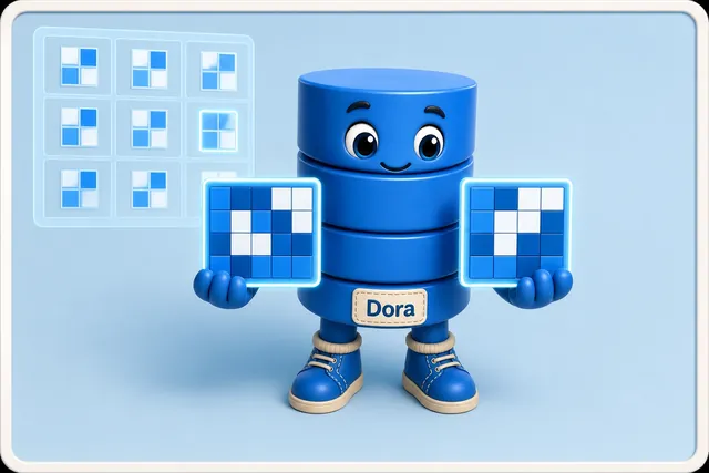
Compare a target block with its best earlier-frame prediction.
-
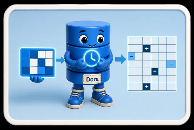
Count how many difference samples remain and how large they are.
-

Choose the cheaper tested mode; an earlier frame does not guarantee a saving.
Suppose a target block differs from its best reference candidate by these signed sample values:
Only five of sixteen residual samples are non-zero and every magnitude is one. That prediction is a strong transform input. If a scene cut instead makes most residual magnitudes large, the motion vector plus residual can cost more than an intra-coded block. A production encoder therefore compares candidate modes; “inter” is not automatically cheaper merely because a previous frame exists.
Data Encoding and Codecs owns the higher-level I/P/B-frame and GOP policy decision. This chapter supplies the lower mechanism: references produce predictions, predictions produce residuals, and residuals still traverse transform, quantization, and lossless packing. Real-Time Protocol Workflows owns the RTP/RTCP hand-off shown at the source diagram’s boundary; it is not re-taught here.
2.3.2 Read Source Rate Ranges as Evidence, Not Targets
The source’s final retained slide compares raw rates with example compressed ranges. These are lecture-era examples, not current codec recommendations. Their value is the scale of the mechanism’s payoff and the reminder that content and encoder settings control the result.
Do not silently repair source data. The still-image row's printed compressed range is larger than its raw image and is labelled MBytes, so it fails its own compression claim. It may have intended kBytes, but this chapter does not guess. A product record should instead measure the actual images, encoder, quality setting, and decoder path.
2.4 Summary
The chapter’s mechanisms form one argument about controlled loss. Psychoacoustic masking first raises a signal-dependent detection threshold, giving an audio coder a reason to place selected error where it is less audible. For images, an DCT reorganizes a block into one DC and 63 AC spatial-frequency coefficients; quantization then creates high-frequency zeros, and JPEG zig-zag order clusters those zeros for run-length and entropy coding. Video adds prediction: motion estimation selects a reference displacement, motion compensation constructs the predicted block, and the residual preserves what that prediction missed.
Those savings are defensible only when the encoder names both the mechanism and its cost. A perceptual threshold can be exceeded, quantization discards detail, and a poor motion predictor can cost more than an intra-coded block. Treat every compression range as a measurement tied to particular content and settings, not as a timeless property of a codec. If the source units contradict the claimed reduction, reject the comparison rather than silently repairing it. That evidence discipline is what connects the audio, image, and video cases.
2.5 Key Takeaway
Media compression becomes explainable when every saving has a mechanism: a perceptual threshold hides selected audio error, a transform concentrates image energy, or a reference frame predicts video content. State the mechanism, the error it introduces, and the evidence that the intended receiver can still use the result.
2.6 See Also
Continue according to the boundary you need to inspect next. Use Data Encoding and Codecs to step outward from transform and prediction mechanics to containers, GOP structure, and codec selection. Choose Voice Compression and Digital Telephony when the open question is speech coding, latency, header budget, or measured call quality. Audio Features for Machine Learning follows a different branch: its time-frequency representation supports classification rather than reconstructable playback. Finally, VoIP Client Architecture places these media operations inside the signaling, processing, packet, and device responsibilities of a complete calling product.
- Data Encoding and Codecs — the codec/container, selection, I/P/B-frame, GOP, and quality-evaluation decision layer this chapter extends.
- Voice Compression and Digital Telephony — PCM, companding, ADPCM/CELP/LPC, quality metrics, and VoIP packet-budget material intentionally not repeated here.
- Audio Features for Machine Learning — a different use of time-frequency decomposition: extracting classification features rather than reconstructable media.
- VoIP Client Architecture: Two Case Studies — how media processing and transport components assemble into a calling product.
Together, these routes separate three questions that should not be collapsed: how a representation saves bits, how the resulting payload behaves on a real-time path, and which product component owns each failure and item of evidence.