Compare LoRaWAN ADR with a fixed spreading factor

Use the module guide's LoRaWAN link-budget and ADR pathway to compare spreading factor, reference airtime and delivered uplinks under changing path loss.

Read delivered uplinks alongside the final rate; require real link evidence before a deployment decision., your practice guide

Read delivered uplinks alongside the final rate; require real link evidence before a deployment decision.
Predict the reading, then compare it with the measurement.

ns-3 with signetlabdei LoRaWAN

Python

Use the module guide's LoRaWAN link-budget and ADR pathway to compare spreading factor, reference airtime and delivered uplinks under changing path loss.

Tier 2 · Python · install required · No account

Version tested: ns-3.48 d2add90b452d600cfb4859baed8e9ea633519447; signetlabdei/lorawan e45b4af428c92f30b2e6c201055809110758125f. Date: 2026-10-08.

Download the lab files, build the pinned ns-3 LoRaWAN module, and run run.sh followed by analyze.py.

Open the Python run guide (new tab)

Get the files

Download all three prepared files into one folder. No account or paid service is required.

README.md

3,199 bytes · Run guide

Download

# Compare ADR with a fixed spreading factor in ns-3

This is a second tool route for the LoRaWAN link-budget and ADR concept. It runs the real `adr-example` in the [signetlabdei LoRaWAN ns-3 module](https://github.com/signetlabdei/lorawan), paired with the same example with ADR disabled. The module simulates **Class A** end devices only. Its output is a model result, **not a radio capture**.

The positions and random path-loss additions are **synthetic** model inputs, with `RngSeed=7` and `RngRun=1`. The source is `examples/adr-example.cc` at LoRaWAN commit `e45b4af428c92f30b2e6c201055809110758125f`. The compatible ns-3 tag `ns-3.48` resolves to commit `d2add90b452d600cfb4859baed8e9ea633519447`. The six conditions use 16 devices, 30 twenty-minute periods, a 4 km half-side placement square, a 5 km gateway spacing and maximum random losses of 0, 10 or 20 dB. `scenario.json` records the inputs.

## Run locally or in a free Linux cloud shell

Use a Linux terminal with a C++ compiler, Git, CMake ≥3.13 and Python 3 with matplotlib. A free cloud shell with these tools works; its CPU and memory limits determine build time. Download `run.sh`, `analyze.py` and `scenario.json` from this lab page into one directory, then run these commands there. No paid ns-3 service or radio hardware is needed.

```bash
git clone --depth 1 --branch ns-3.48 https://gitlab.com/nsnam/ns-3-dev.git ns-3-dev
test "$(git -C ns-3-dev rev-parse HEAD)" = d2add90b452d600cfb4859baed8e9ea633519447
git clone https://github.com/signetlabdei/lorawan.git ns-3-dev/src/lorawan
git -C ns-3-dev/src/lorawan checkout e45b4af428c92f30b2e6c201055809110758125f
test "$(git -C ns-3-dev/src/lorawan rev-parse HEAD)" = e45b4af428c92f30b2e6c201055809110758125f
(cd ns-3-dev && ./ns3 configure --enable-examples --enable-modules lorawan && ./ns3 build -j 8)
bash run.sh "$PWD/ns-3-dev" "$PWD/results"
python3 analyze.py "$PWD/results"
```

On Debian or Ubuntu, `sudo apt install g++ python3 python3-matplotlib cmake git` supplies the listed dependencies. On a managed cloud shell, use its preinstalled compiler and Python packages if package installation is unavailable. The build uses no more than eight jobs.

`run.sh` writes six directories under `results/`. Each has the real simulator's `stdout.log`, `nodeData.txt` and `globalPerformance.txt`. `analyze.py` reads these outputs, prints the six rows, writes `summary.csv` and renders `delivery.png`. Open that PNG in a browser. The 10-byte **reference** airtime is calculated from each run's final spreading factors using the module's time-on-air formula and stated PHY assumptions; it is **not a measurement of the actual LoRaWAN uplink frame or of all packets across the run**. Delivery uses the module's global MAC packet tracker across the run. The example's final console line covers only the final 20-minute window.

Expected output for this pinned, fixed-seed run is in `expected-summary.csv`; compare your own CSV with it. Small differences after changing versions, seeds or parameters require a fresh evidence record rather than editing expected values.

The result does not establish real-world coverage, battery life, or a good ADR policy for a field deployment.

run.sh

891 bytes · Run guide

Download

analyze.py

2,828 bytes · Run guide

Download

#!/usr/bin/env python3
"""Reduce the real adr-example outputs and plot final rate versus delivery."""
import csv
import math
from pathlib import Path
import sys

from matplotlib import pyplot as plt

def reference_airtime_ms(sf):
    # Module LoraPhy::GetTimeOnAir formula for a 10-byte reference PHY frame.
    symbol_s = 2**sf / 125000
    low_rate_opt = int(sf >= 11)
    symbols = 8 + max(math.ceil((80 - 4 * sf + 28 + 16) / (4 * (sf - 2 * low_rate_opt))) * 5, 0)
    return round(((8 + 4.25) + symbols) * symbol_s * 1000, 2)

def read_case(case_dir):
    statuses = [line.split() for line in (case_dir / "nodeData.txt").read_text().splitlines()]
    last_time = statuses[-1][0]
    final = [line for line in statuses if line[0] == last_time]
    drs = [int(line[4]) for line in final]
    perf = [line.split() for line in (case_dir / "globalPerformance.txt").read_text().splitlines()]
    sent = sum(int(float(line[1])) for line in perf)
    received = sum(int(float(line[2])) for line in perf)
    sf = [12 - dr for dr in drs]
    return sent, received, round(sum(sf) / len(sf), 2), round(sum(reference_airtime_ms(s) for s in sf) / len(sf), 2), min(sf), max(sf)

def main(result_dir):
    rows = []
    for loss in (0, 10, 20):
        for mode in ("adr", "fixed"):
            sent, delivered, mean_sf, airtime, min_sf, max_sf = read_case(result_dir / f"{mode}-loss{loss}")
            rows.append(dict(loss_db=loss, mode=mode, sent=sent, delivered=delivered,
                             delivery_pct=round(100 * delivered / sent, 1),
                             mean_final_sf=mean_sf, min_final_sf=min_sf, max_final_sf=max_sf,
                             reference_airtime_ms=airtime))
    with (result_dir / "summary.csv").open("w", newline="") as out:
        writer = csv.DictWriter(out, fieldnames=rows[0].keys(), lineterminator="\n")
        writer.writeheader()
        writer.writerows(rows)
    for row in rows:
        print(f"loss={row['loss_db']:2} mode={row['mode']:5} delivered={row['delivered']:3}/{row['sent']:3} ({row['delivery_pct']:5.1f}%) final_SF={row['mean_final_sf']:5.2f} [{row['min_final_sf']}-{row['max_final_sf']}] reference_airtime={row['reference_airtime_ms']:7.2f} ms")
    fig, ax = plt.subplots(figsize=(8, 4.5))
    for mode, marker in (("adr", "o"), ("fixed", "s")):
        subset = [row for row in rows if row["mode"] == mode]
        ax.plot([r["loss_db"] for r in subset], [r["delivery_pct"] for r in subset], marker=marker, label=mode.upper())
    ax.set(xlabel="Maximum synthetic random loss (dB)", ylabel="Delivered uplinks (%)", ylim=(0, 105), xticks=[0, 10, 20])
    ax.grid(alpha=0.3)
    ax.legend()
    fig.tight_layout()
    fig.savefig(result_dir / "delivery.png", dpi=150)

if __name__ == "__main__":
    main(Path(sys.argv[1] if len(sys.argv) > 1 else "results"))

scenario.json

635 bytes · Run guide

Download

expected-summary.csv

324 bytes · Run guide

Download

Put main.py, requirements.txt, and README.md in the same folder.
Create and activate a Python virtual environment, then install requirements.txt.
Run python3 main.py and compare its output with each observed result below.

Steps

Screens captured against ns-3 adr-example in XFCE terminal; Firefox plot view ns-3.48 and signetlabdei/lorawan e45b4af on 2026-10-08; the tool may have moved on — the text steps are the contract.

Step 1
Do
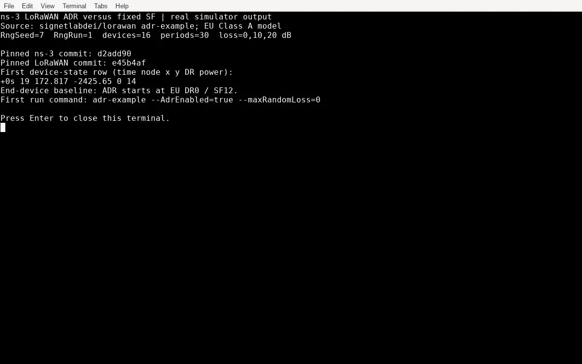
In the terminal panel, follow README.md to pin and build ns-3 and the LoRaWAN module. Check the two commits, then run all six cases with run.sh. Read the first row in results/adr-loss0/nodeData.txt.
You will see
The tested commits are ns-3 d2add90 and LoRaWAN e45b4af. At simulated 0 s, one device row has DR0 and 14 dBm; EU DR0 maps to SF12. The positions and loss draw are synthetic, with RngSeed=7 and RngRun=1.
Why it matters
The version, seed and starting data rate make every later comparison traceable to the actual model run.
Step 2
Do
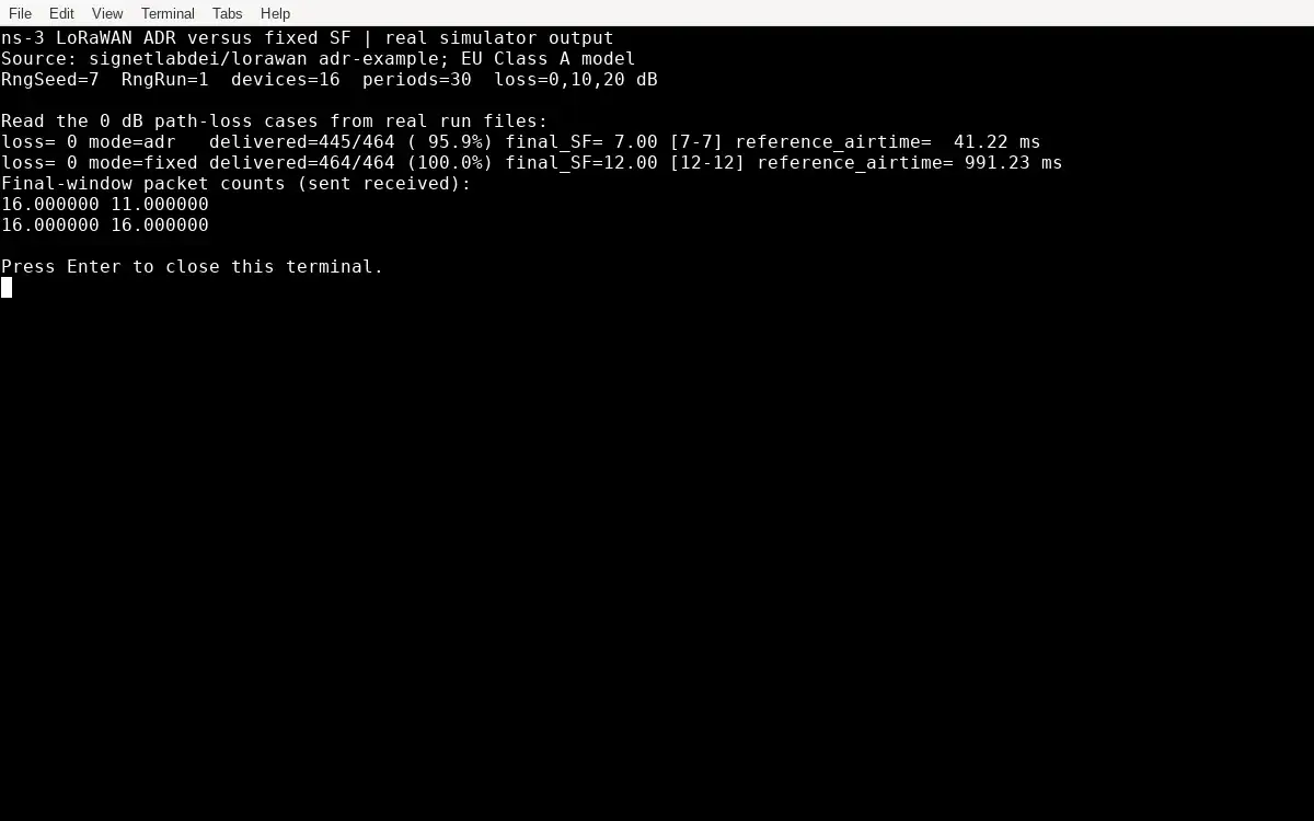
In the terminal panel, compare the 0 dB ADR and fixed rows printed by analyze.py. Read each case's final-window line in stdout.log. Keep full-run delivery separate from that last-window count.
You will see
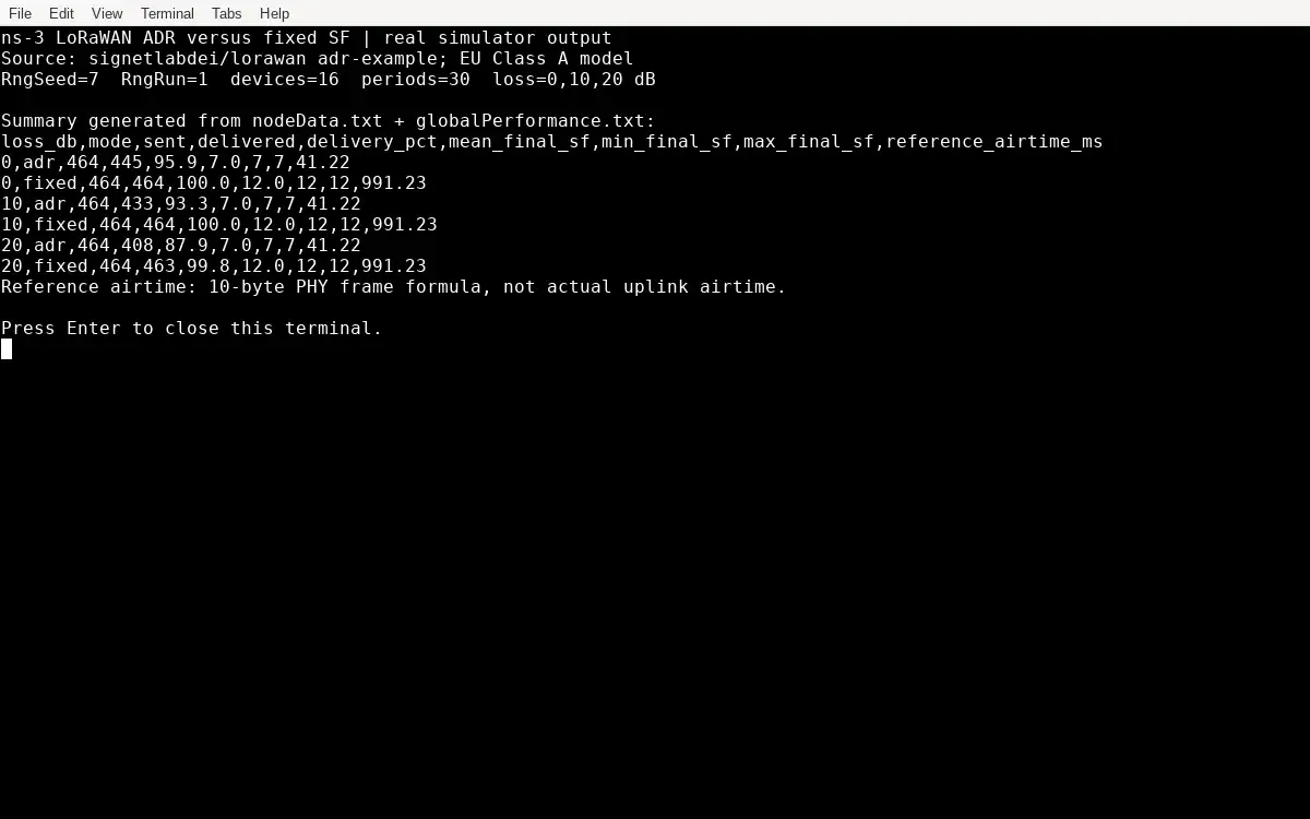
At 0 dB, ADR delivers 445/464 uplinks (95.9%); fixed SF12 delivers 464/464 (100.0%). The final observed ADR spreading factor is SF7 for all 16 devices. The last 20-minute window reports 11/16 for ADR and 16/16 for fixed.
Why it matters
ADR is faster at the final observed setting, but the complete-run delivery record already shows a tradeoff.
Step 3
Do
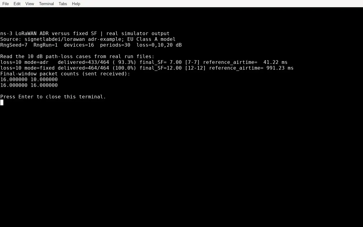
In the terminal panel, read the paired 10 dB loss rows and their stdout.log tails. Check the same RngSeed=7 and RngRun=1 in run.sh. Compare delivered packets before discussing airtime.
You will see
At 10 dB, ADR delivers 433/464 (93.3%); fixed SF12 delivers 464/464 (100.0%). The final observed ADR rate remains SF7, while fixed remains SF12. The last window reports 10/16 for ADR and 16/16 for fixed.
Why it matters
The paired input isolates the effect of enabling ADR in this synthetic path-loss condition.
Step 4
Do
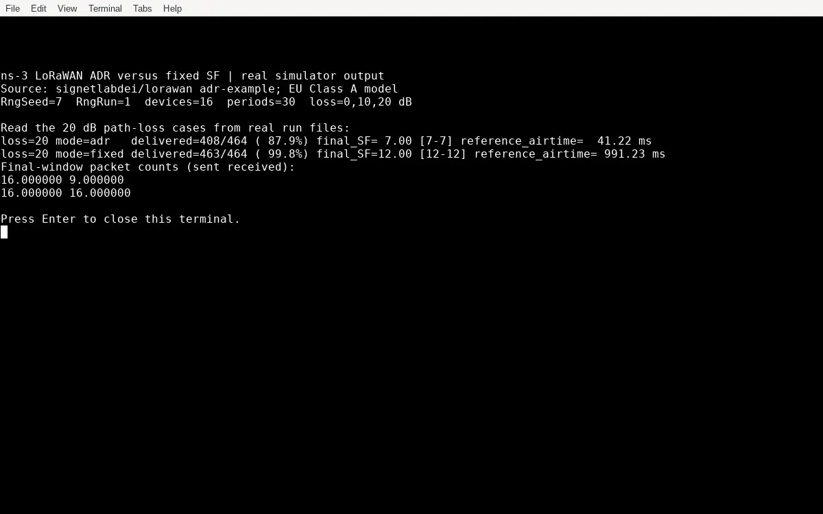
In the terminal panel, inspect the 20 dB rows and final-window counts. Compare both modes against their 0 dB cases. Record whether the chosen final spreading factors changed.
You will see
At 20 dB, ADR delivers 408/464 (87.9%); fixed SF12 delivers 463/464 (99.8%). The final observed settings remain SF7 and SF12 respectively. The last window reports 9/16 for ADR and 16/16 for fixed. In the 20 dB ADR trace, device 26 has 20 received SNRs from -11.755 to +7.21097 dB; the default uses their maximum.
Why it matters
The loss sweep shows the delivery cost of this ADR outcome as modeled conditions become harsher. The strongest received packet can outweigh weaker ones when random loss changes between uplinks.
Step 5
Do
In the terminal panel, inspect results/summary.csv made by analyze.py. Compare mean final SF and the 10-byte reference airtime across all six rows. Mark the reference as a formula result, not recorded frame airtime.
You will see
Every ADR row ends at mean SF7; every fixed row ends at SF12. The corresponding 10-byte reference airtimes are 41.22 ms and 991.23 ms. The CSV keeps all six full-run delivery ratios beside these final-setting references. For device 26, max SNR 7.21097 minus the SF12 threshold -20.0 gives a 27.21097 dB margin; floor(27.21097/3)=9 steps. Five steps take SF12 to SF7; four more take transmit power from 14 to 6 dBm.
Why it matters
A shorter reference airtime describes the rate tradeoff without pretending to measure actual uplink airtime or battery life. Pinned source: adr-component.cc:207 `double margin_SNR = m_SNR - req_SNR;`; :213 `int steps = std::floor(margin_SNR / 3);`. The source uses no separate device-margin offset: adr-component.h:160 comments it out. Pinned adr-component.h:160 `// const int offset = 10; //!< Device specific SNR margin (dB)`.
Step 6
Do
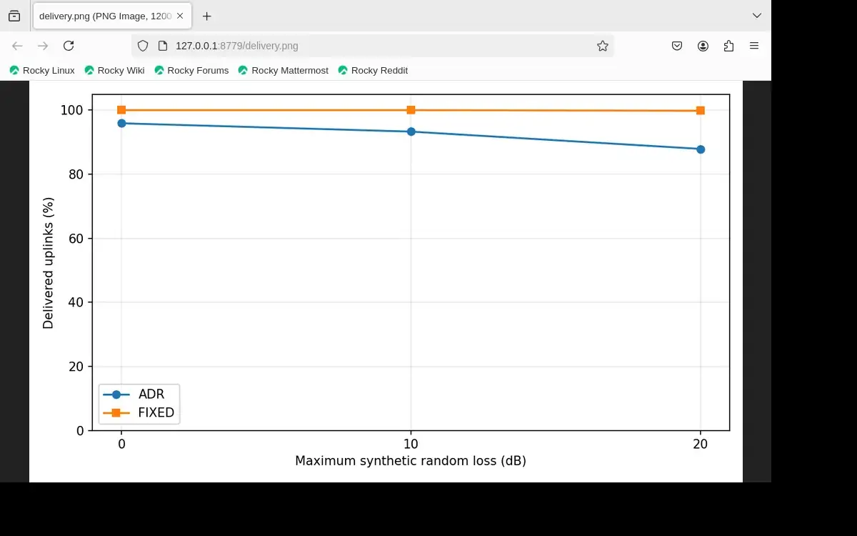
In the browser tab, open the delivery.png plot generated from your run's summary.csv. Trace the ADR and fixed lines from 0 to 20 dB. Write a decision that includes both the airtime reference and lost uplinks.
You will see
The ADR line declines from 95.9% to 93.3% to 87.9%. The fixed SF12 line is 100.0%, 100.0% and 99.8%. All points come from the six ns-3 runs, not a hand-drawn result panel. Pinned defaults: adr-component.cc:46 `EnumValue(AdrComponent::MAXIMUM),`; :56 `IntegerValue(20),`. The SF12 and SF7 required SNRs are -20.0 and -7.5 dB (adr-component.h:164,169). Pinned adr-component.h:164 `-20.0,` and :169 `-7.5}; //!< Vector containing the required SNR for the 6 allowed spreading factor`. Pinned adr-component.cc:182 `m_SNR = GetMaxSNR(status->GetReceivedPacketList(), historyRange);`.
Why it matters
The plot supports a bounded model comparison; it cannot select a field ADR policy without measured links and deployment requirements. Selecting the best of 20 received packets overlooks weaker receptions and packets that did not arrive; changing synthetic loss can therefore make SF7 lose later uplinks. SF7 has about 24 times less 10-byte reference airtime than SF12, but this run delivers fewer packets under fluctuating loss. A deployment could test the exposed history statistic or range (adr-component.cc:44-58) against measured links before setting its policy.

Chapter checks

These questions refer to the chapter’s examples. Use the return links to review their answers.

Before enabling ADR for a planned LoRaWAN sensor route, which evidence belongs in the link-budget record?
Return to the chapter’s knowledge check
A device has one excellent uplink and several weak uplinks from the same installation. What should the reviewer do before approving a less robust setting?
Return to the chapter’s knowledge check

Return to LoRaWAN Link Budget and ADR · Browse Labs

ns-3 with signetlabdei LoRaWAN

Get the files

README.md

run.sh

analyze.py

scenario.json

expected-summary.csv

Steps

1 Step 1

2 Step 2

3 Step 3

4 Step 4

5 Step 5

6 Step 6

Chapter checks

Step 1

Step 2

Step 3

Step 4

Step 5

Step 6