Calculate LoRaWAN airtime and Class A receive-window budgets
Calculate how spreading factor, payload size and report interval affect modeled airtime and Class A receive-window timing.

Use the LoRaWAN operations chapter to prepare and review evidence for device-class timing and slow-data-rate payload decisions.
Predict the reading, then compare it with the measurement.
Python 3 in your browser (JupyterLite)
Python · no installCalculate how spreading factor, payload size and report interval affect modeled airtime and Class A receive-window timing.
Open the notebook in your browser and run each Python cell; no install or account is needed.
Three ways to run: use JupyterLite here with no install; run main.py locally from the downloadable lab folder; or open the same notebook in Google Colab.
Steps
Step 1
- Do
- In the notebook editor, run the Step 1 notebook cell. Freeze the hypothetical LoRa radio inputs.
- You will see
- The run prints 21 PHYPayload bytes, 125000 Hz bandwidth, coding rate 4/5 and eight preamble symbols.
- Why it matters
- A timing result needs its framing assumptions.
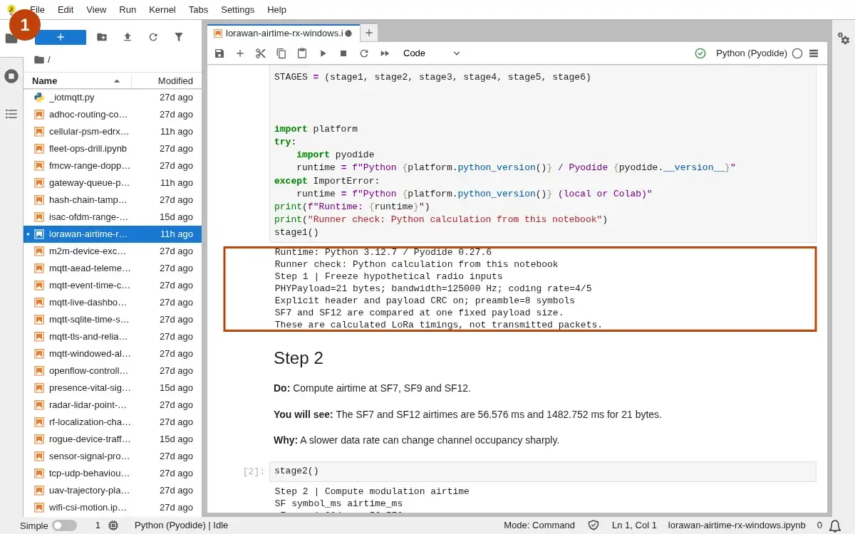
Step 1 · Python 3 in your browser (JupyterLite); numbered callout added to a real capture. Enlarge screenshot (new tab) Step 2
- Do
- In the notebook editor, run the Step 2 notebook cell. Compute airtime at SF7, SF9 and SF12.
- You will see
- The SF7 and SF12 airtimes are 56.576 ms and 1482.752 ms for 21 bytes.
- Why it matters
- A slower data rate can change channel occupancy sharply.
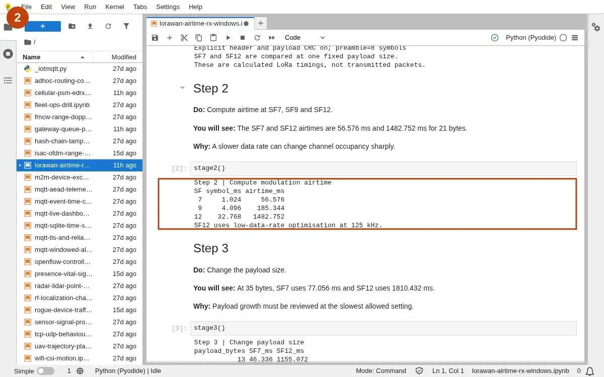
Step 2 · Python 3 in your browser (JupyterLite); numbered callout added to a real capture. Enlarge screenshot (new tab) Step 3
- Do
- In the notebook editor, run the Step 3 notebook cell. Change the payload size.
- You will see
- At 35 bytes, SF7 uses 77.056 ms and SF12 uses 1810.432 ms.
- Why it matters
- Payload growth must be reviewed at the slowest allowed setting.
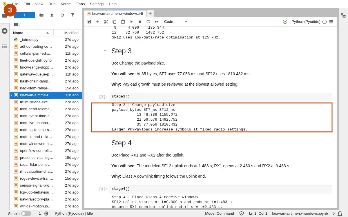
Step 3 · Python 3 in your browser (JupyterLite); numbered callout added to a real capture. Enlarge screenshot (new tab) Step 4
- Do
- In the notebook editor, run the Step 4 notebook cell. Place RX1 and RX2 after the uplink.
- You will see
- The modeled SF12 uplink ends at 1.483 s; RX1 opens at 2.483 s and RX2 at 3.483 s.
- Why it matters
- Class A downlink timing follows the uplink end.
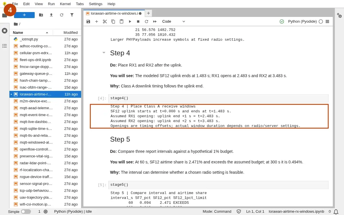
Step 4 · Python 3 in your browser (JupyterLite); numbered callout added to a real capture. Enlarge screenshot (new tab) Step 5
- Do
- In the notebook editor, run the Step 5 notebook cell. Compare three report intervals against a hypothetical 1% budget.
- You will see
- At 60 s, SF12 airtime share is 2.471% and exceeds the assumed budget; at 300 s it is 0.494%.
- Why it matters
- The interval can determine whether a chosen radio setting is feasible.
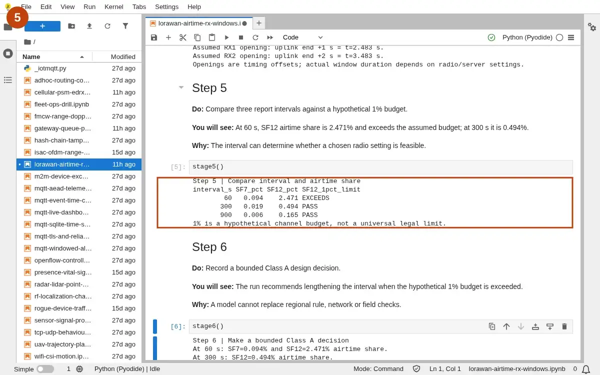
Step 5 · Python 3 in your browser (JupyterLite); numbered callout added to a real capture. Enlarge screenshot (new tab) Step 6
- Do
- In the notebook editor, run the Step 6 notebook cell. Record a bounded Class A design decision.
- You will see
- The run recommends lengthening the interval when the hypothetical 1% budget is exceeded.
- Why it matters
- A model cannot replace regional rule, network or field checks.
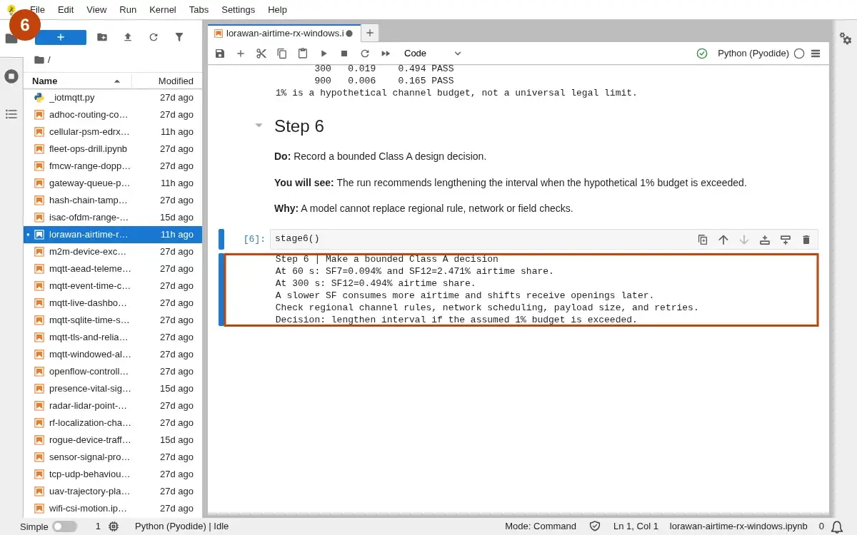
Step 6 · Python 3 in your browser (JupyterLite); numbered callout added to a real capture. Enlarge screenshot (new tab)
Chapter checks
These questions refer to the chapter’s examples. Use the return links to review their answers.
A LoRaWAN deployment has missing readings after devices move from the lab bench to final placement. Which first review step keeps the diagnosis bounded?
Return to the chapter’s knowledge checkA payload works near the gateway but fails after final installation when the network selects a slower data rate. What is the best review response?
Return to the chapter’s knowledge check