Duty-cycle energy and latency budget
Build an energy-latency budget from components and explain when duty cycling helps or hurts.
Build an energy-latency budget from components and explain when duty cycling helps or hurts.
Predict the reading, then compare it with the measurement.
Python 3 in your browser (JupyterLite)
Python · no installBuild an energy-latency budget from components and explain when duty cycling helps or hurts.
Open the notebook in your browser and run each Python cell; no install or account is needed.
Three ways to run: use JupyterLite here with no install; run main.py locally from the downloadable lab folder; or open the same notebook in Google Colab.
Steps
Step 1
- Do
- Run the Step 1 notebook cell to inspect the labelled synthetic current and timing assumptions.
- You will see
- SYNTHETIC engineering assumptions; seed=2626; no random draws; supply=3.0 V; active=8.00 mA for 100 ms; radio=35.00 mA for 80 ms per attempt; sleep=0.040 mA; retry adds 80 ms radio-on; latency limit=300 ms; daily energy limit=30 J
- Why it matters
- Every estimate must reveal its units and assumed inputs.
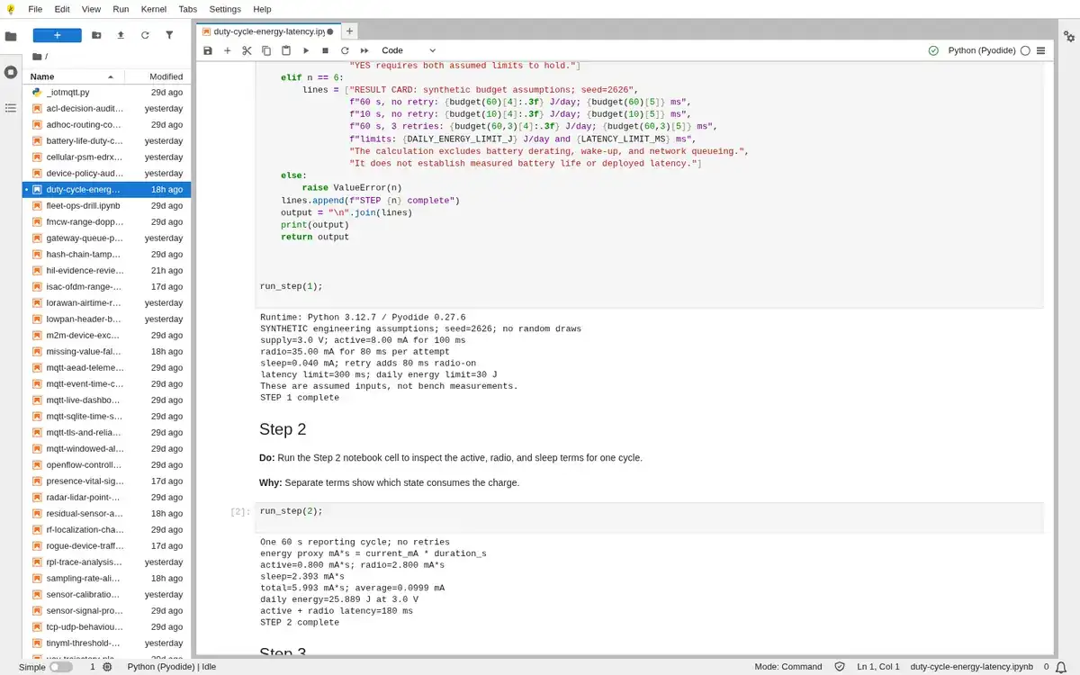
Step 1 · Python 3 in your browser (JupyterLite); numbered callout added to a real capture. Enlarge screenshot (new tab) Step 2
- Do
- Run the Step 2 notebook cell to inspect the active, radio, and sleep terms for one cycle.
- You will see
- One 60 s reporting cycle; no retries; energy proxy mA*s = current_mA * duration_s; daily energy=25.889 J at 3.0 V; active + radio latency=180 ms
- Why it matters
- Separate terms show which state consumes the charge.
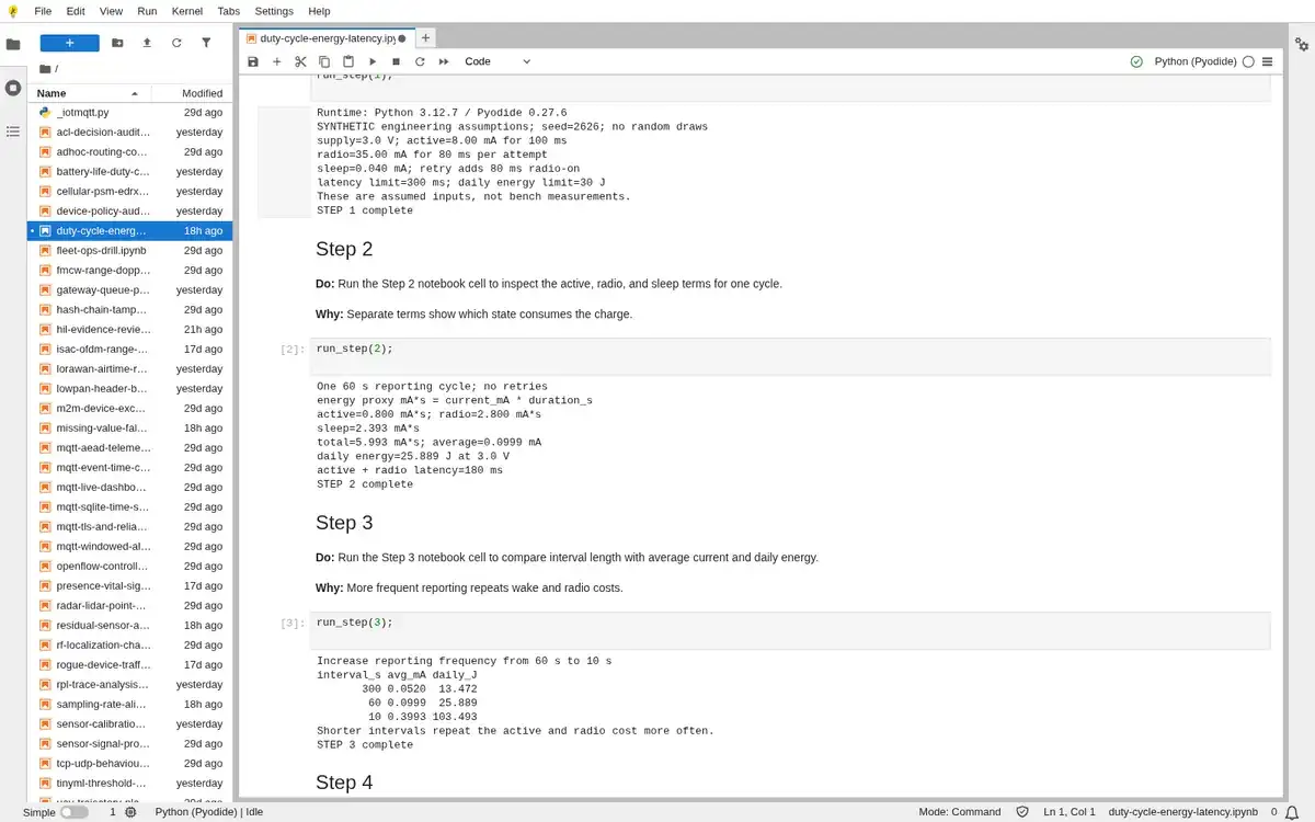
Step 2 · Python 3 in your browser (JupyterLite); numbered callout added to a real capture. Enlarge screenshot (new tab) Step 3
- Do
- Run the Step 3 notebook cell to compare interval length with average current and daily energy.
- You will see
- Increase reporting frequency from 60 s to 10 s; interval_s avg_mA daily_J; 10 0.3993 103.493; Shorter intervals repeat the active and radio cost more often.
- Why it matters
- More frequent reporting repeats wake and radio costs.
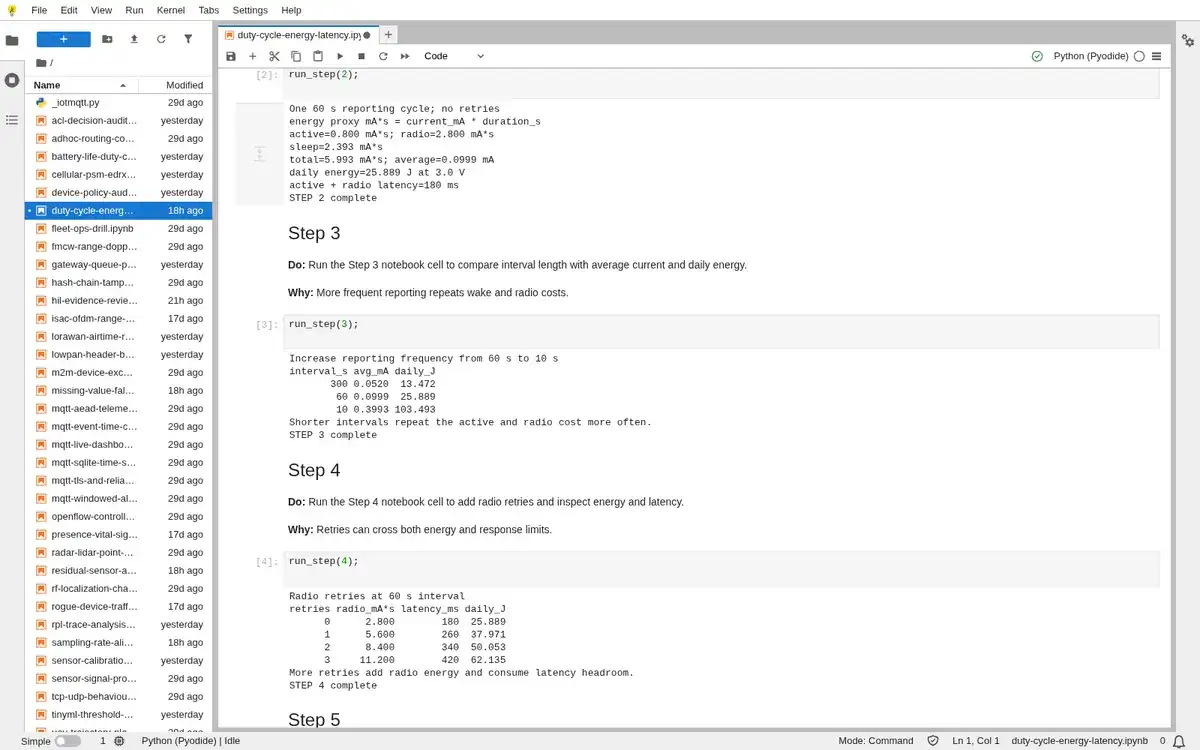
Step 3 · Python 3 in your browser (JupyterLite); numbered callout added to a real capture. Enlarge screenshot (new tab) Step 4
- Do
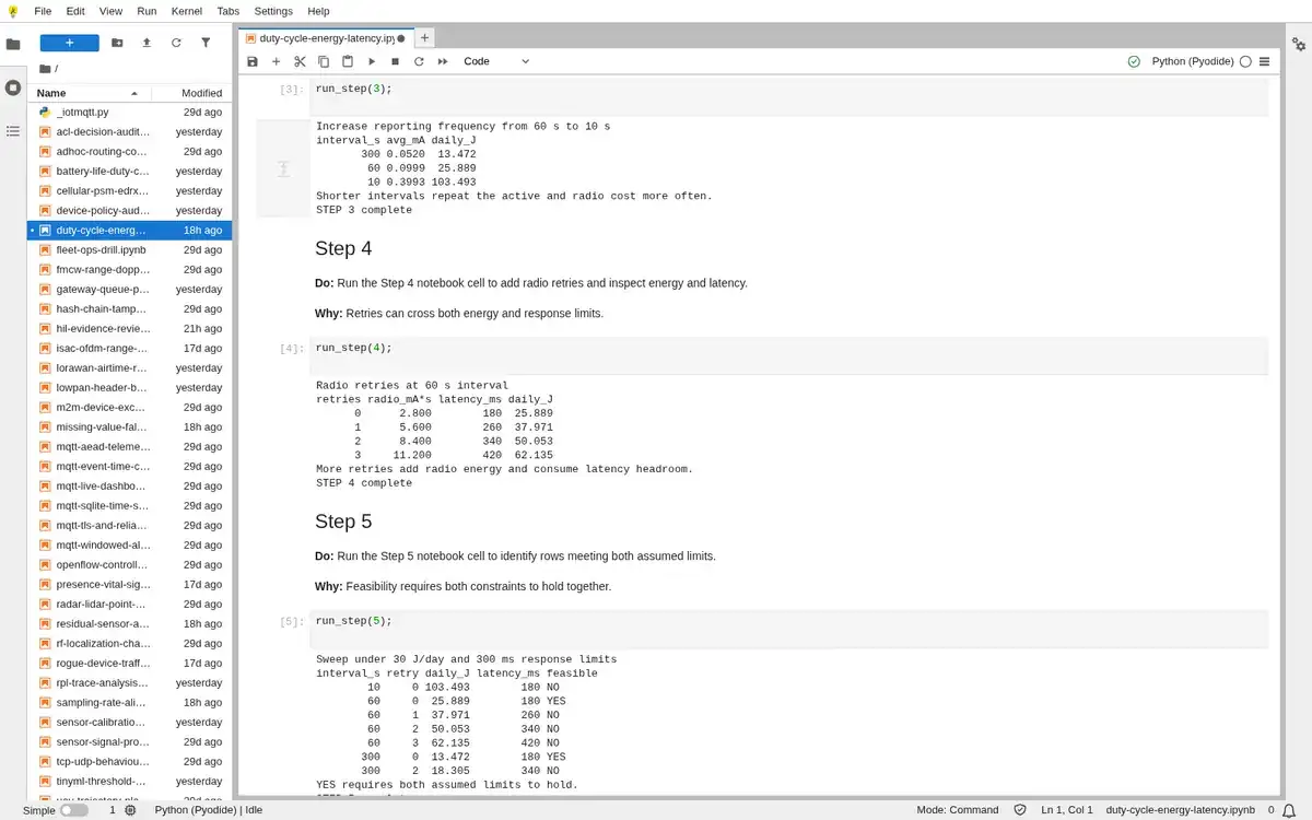
- Run the Step 4 notebook cell to add radio retries and inspect energy and latency.
- You will see
- Radio retries at 60 s interval; retries radio_mA*s latency_ms daily_J; 3 11.200 420 62.135; More retries add radio energy and consume latency headroom.
- Why it matters
- Retries can cross both energy and response limits.
Step 4 · Python 3 in your browser (JupyterLite); numbered callout added to a real capture. Enlarge screenshot (new tab) Step 5
- Do
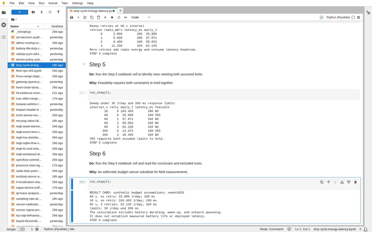
- Run the Step 5 notebook cell to identify rows meeting both assumed limits.
- You will see
- Sweep under 30 J/day and 300 ms response limits; interval_s retry daily_J latency_ms feasible; 300 2 18.305 340 NO; YES requires both assumed limits to hold.
- Why it matters
- Feasibility requires both constraints to hold together.
Step 5 · Python 3 in your browser (JupyterLite); numbered callout added to a real capture. Enlarge screenshot (new tab) Step 6
- Do
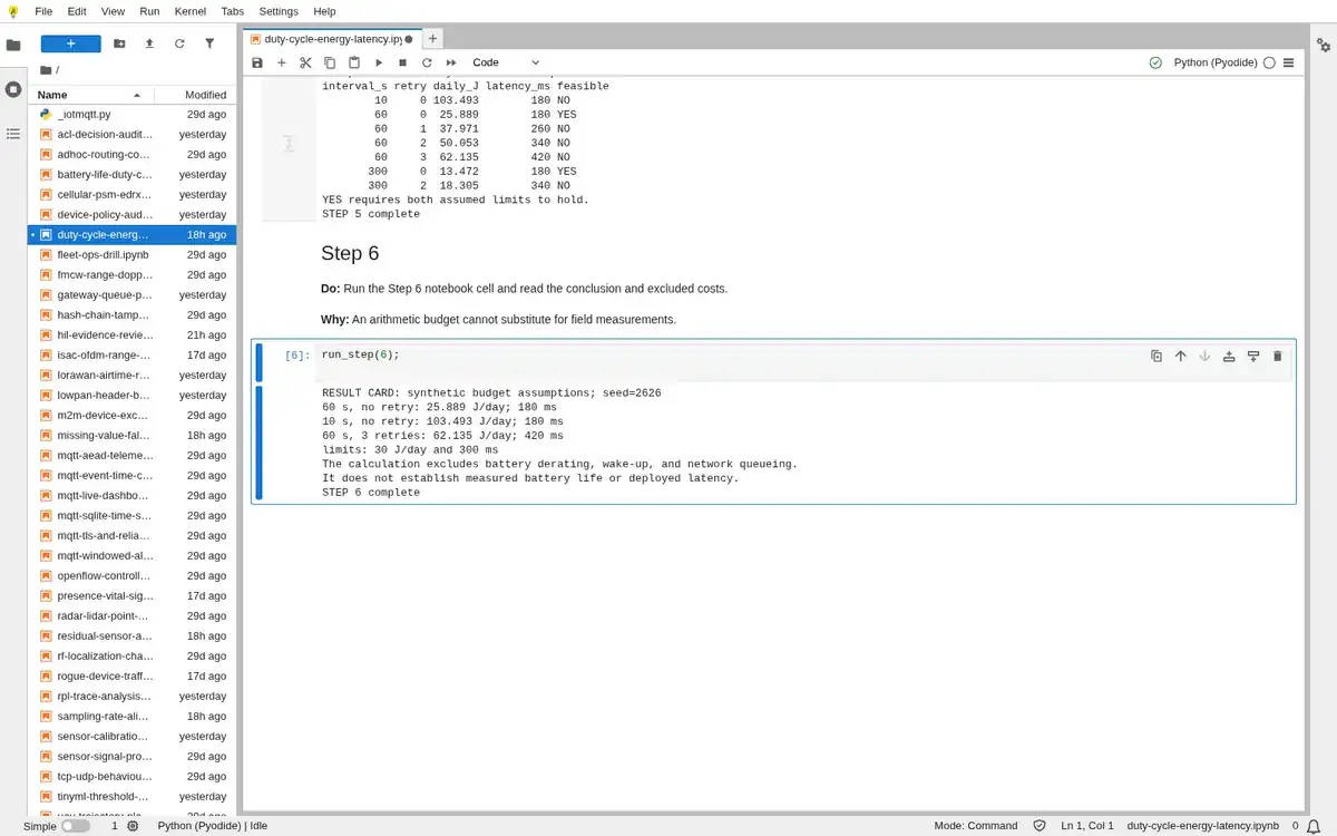
- Run the Step 6 notebook cell and read the conclusion and excluded costs.
- You will see
- RESULT CARD: synthetic budget assumptions; seed=2626; 60 s, no retry: 25.889 J/day; 180 ms; The calculation excludes battery derating, wake-up, and network queueing.; It does not establish measured battery life or deployed latency.
- Why it matters
- An arithmetic budget cannot substitute for field measurements.
Step 6 · Python 3 in your browser (JupyterLite); numbered callout added to a real capture. Enlarge screenshot (new tab)
Chapter checks
These questions refer to the chapter’s examples. Use the return links to review their answers.
Why does this chapter say fog computing is not automatically faster, cheaper, or lower power?
Return to the chapter’s knowledge checkA fog node compresses routine data before upload. What measurement decides whether this helps overall?
Return to the chapter’s knowledge check