Budget battery life from duty cycle
Turn the module guide's battery-life and measurement path into an auditable duty-cycle sensitivity budget.

Inspect the measured current terms and the datasheet condition before trusting a lifetime number.
Predict the reading, then compare it with the measurement.
Python 3 in your browser (JupyterLite)
Python · no installTurn the module guide's battery-life and measurement path into an auditable duty-cycle sensitivity budget.
Open the notebook in your browser and run each Python cell; no install or account is needed.
Three ways to run: use JupyterLite here with no install; run main.py locally from the downloadable lab folder; or open the same notebook in Google Colab.
Steps
Step 1
- Do
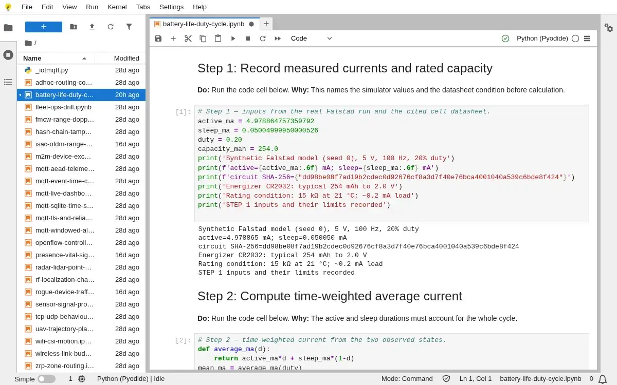
- Run the first code cell in the JupyterLite notebook editor and inspect the input record.
- You will see
- Synthetic Falstad model (seed 0), 5 V, 100 Hz, 20% duty. active=4.978865 mA; sleep=0.050050 mA. Energizer CR2032: typical 254 mAh to 2.0 V. Rating condition: 15 kΩ at 21 °C; ~0.2 mA load. STEP 1 inputs and their limits recorded
- Why it matters
- The capacity rating condition and measured current source limit what this calculation can claim.
Step 1 · Python 3 in your browser (JupyterLite); numbered callout added to a real capture. Enlarge screenshot (new tab) Step 2
- Do
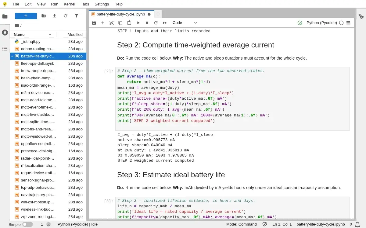
- Run the second code cell in the notebook editor and inspect the weighted-current calculation.
- You will see
- I_avg = duty*I_active + (1-duty)*I_sleep. active share=0.995773 mA. sleep share=0.040040 mA. at 20% duty: I_avg=1.035813 mA. STEP 2 weighted current computed
- Why it matters
- A full-cycle current budget must weight each state by its duration.
Step 2 · Python 3 in your browser (JupyterLite); numbered callout added to a real capture. Enlarge screenshot (new tab) Step 3
- Do
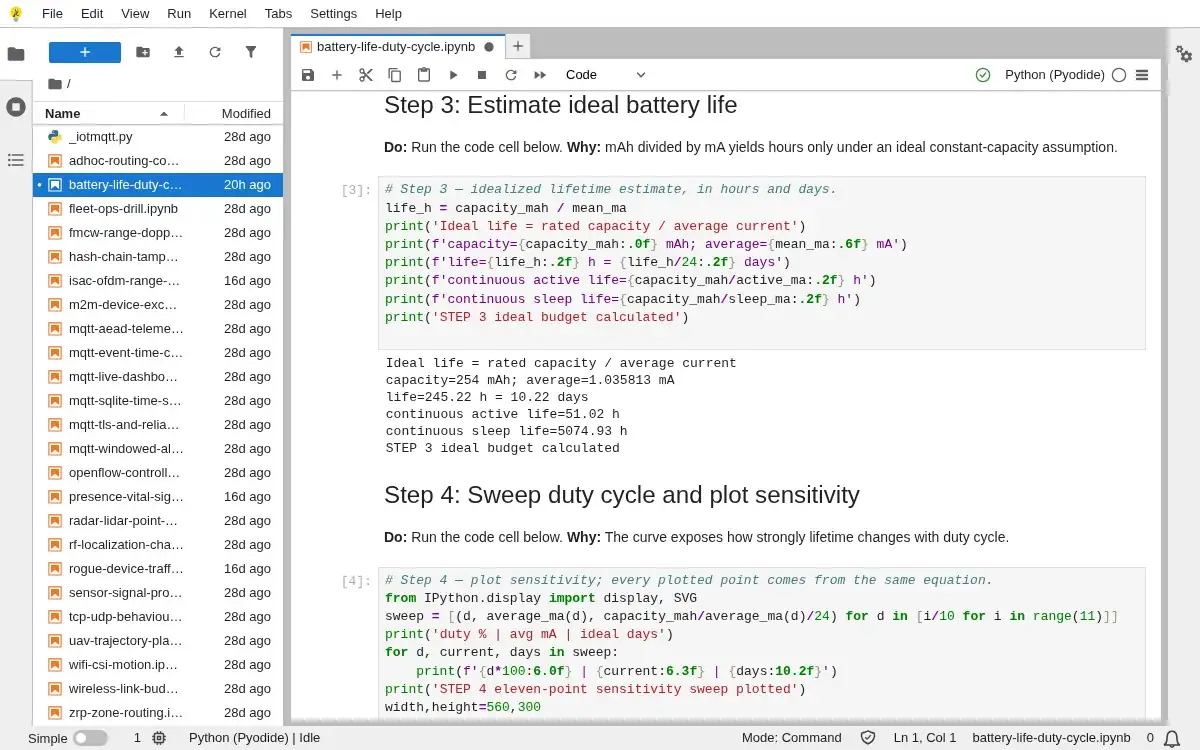
- Run the third code cell in the notebook editor and inspect the ideal-life estimate.
- You will see
- Ideal life = rated capacity / average current. capacity=254 mAh; average=1.035813 mA. life=245.22 h = 10.22 days. continuous active life=51.02 h; continuous sleep=5074.93 h. STEP 3 ideal budget calculated
- Why it matters
- The ideal division gives a screening estimate in hours, with no pulse-load correction.
Step 3 · Python 3 in your browser (JupyterLite); numbered callout added to a real capture. Enlarge screenshot (new tab) Step 4
- Do
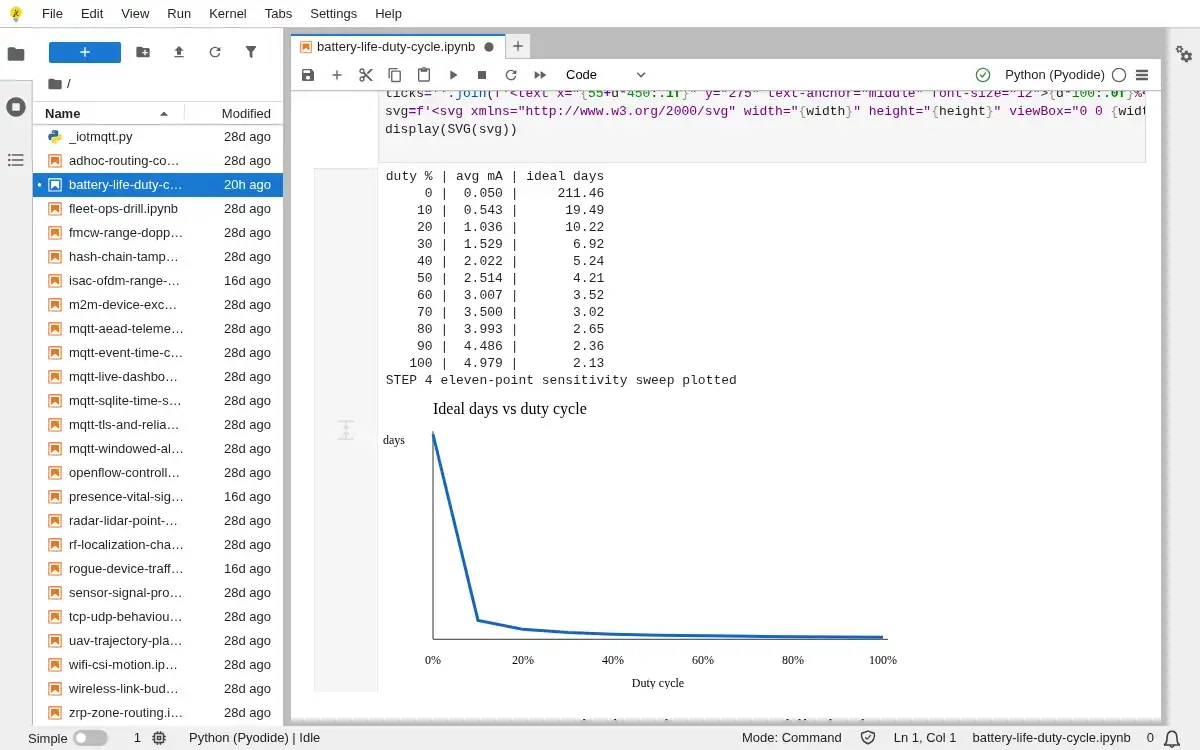
- Run the fourth code cell in the notebook editor and inspect the sweep table and plotted curve.
- You will see
- duty % | avg mA | ideal days 0 | 0.050 | 211.46 10 | 0.543 | 19.49 20 | 1.036 | 10.22 30 | 1.529 | 6.92 40 | 2.022 | 5.24 50 | 2.514 | 4.21 60 | 3.007 | 3.52 70 | 3.500 | 3.02 80 | 3.993 | 2.65 90 | 4.486 | 2.36 100 | 4.979 | 2.13 STEP 4 eleven-point sensitivity sweep plotted
- Why it matters
- Changing duty across eleven cases shows sensitivity beyond one nominal point.
Step 4 · Python 3 in your browser (JupyterLite); numbered callout added to a real capture. Enlarge screenshot (new tab) Step 5
- Do
- Run the fifth code cell in the notebook editor and compare the design changes.
- You will see
- baseline=10.22 days at 20% duty. half sleep current=10.42 days. half active current=19.67 days. half usable capacity=5.11 days. Capacity rating condition differs from this ~1 mA model. STEP 5 sensitivity and boundary compared
- Why it matters
- The dominant current term and usable capacity bound the decision.
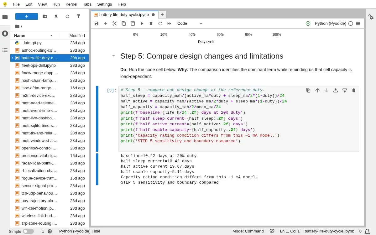
Step 5 · Python 3 in your browser (JupyterLite); numbered callout added to a real capture. Enlarge screenshot (new tab)
Chapter checks
These questions refer to the chapter’s examples. Use the return links to review their answers.
A battery-life calculator predicts four years, but the model uses datasheet sleep current, nominal battery capacity, and one successful radio transmission per cycle. What should the engineer do before accepting the result?
Return to the chapter’s knowledge checkBeyond a single lifetime figure, what is the most useful thing a battery-life tool provides?
Return to the chapter’s knowledge check