← Back to the chapter · Previous detail · Next detail →
Technical detail · Measure-First Optimization
Voltage scaling and dynamic energy
Race-to-sleep assumed the higher clock ran at the same voltage. Often it cannot. Dynamic power scales with the square of the supply voltage as well as with frequency, so if reaching a higher clock requires raising the core voltage, the dynamic energy that was previously constant now grows with voltage squared. A 20% voltage increase multiplies the dynamic energy by about 1.44, which can wipe out the fixed-overhead saving. In the worked example, a 20% voltage increase raises dynamic energy from 1.20 mJ to 1.728 mJ and the 2 mA overhead energy to 0.400 mJ, for a 2.128 mJ 48 MHz total - now barely better than the 2.20 mJ slow-clock baseline, and worse at larger voltage steps.
Use Figure 16.1 to test whether a faster operating point still saves cycle energy after voltage-squared switching power, execution time, and idle break-even are included.
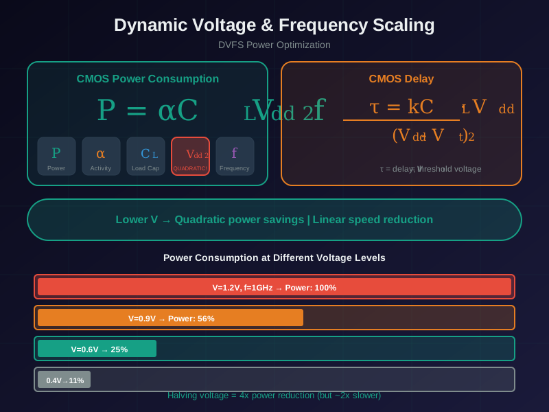
Read Figure 16.1 from the switching-power relation P ∝ V²f to execution time and then active energy. Raising frequency shortens the task, but any required voltage increase is squared in the dynamic term. At 1.3 V instead of 1.0 V, that multiplier is 1.3² = 1.69; the 1.20 mJ dynamic energy becomes 2.028 mJ, while dynamic charge becomes 1.56 mA·s, before fixed overhead. The break-even view then asks whether the resulting idle interval repays the transition. Measured rail energy and achieved sleep, not frequency alone, decide the operating point.
The mathematical gist. A switched node pays joules per charge-discharge cycle, so changing a rail from 1.0 V to 1.3 V multiplies dynamic energy by . At 1.0 V, the 1.20 mA-s charge baseline is 1.20 mJ; at 1.3 V, dynamic energy becomes 2.028 mJ while dynamic charge becomes 1.56 mA-s, while a 15 pF node rises from 15.0 pJ to 25.35 pJ per cycle.