26 Smart Parking Sensor Contracts
26.1 Start With the Story
Begin with a driver searching for a space and a city trying to manage curbside demand. This contract chapter turns smart parking into an evidence chain: detect occupancy, prove confidence, publish availability, guide action, and define what happens when the sensor, network, or payment context is wrong.

Phoebe’s Why
The in-ground sensor never measures a car; it measures a magnetic field, and the field-to-voltage step is a Hall-effect junction. Push a steady current through a thin conductive slab and apply a magnetic field perpendicular to it, and the moving charge carriers feel a sideways Lorentz force, \(F=qv\times B\). Carriers pile up on one edge until the electric field they build up pushes back exactly as hard as the magnetic force – equilibrium – and that sideways electric field, integrated across the slab’s width, is the Hall voltage the sensor actually reads. A car’s steel body does not touch the sensor; it just bends the ambient field passing through this one junction, and the junction inverts that bend back into a number.
The Derivation
At equilibrium, the transverse electric force balances the magnetic force on each carrier:
\[qE_H = qv_d B \implies E_H = v_d B\]
Current relates to carrier density \(n\), drift velocity \(v_d\), and cross-section (width \(w\), thickness \(t\)):
\[I = nqv_d(wt) \implies v_d = \frac{I}{nqwt}\]
Substituting and multiplying by width \(w\) to get the Hall voltage \(V_H=E_H w\), the width cancels:
\[V_H = \frac{I\,B}{n\,q\,t} = \frac{R_H\,I\,B}{t}, \qquad R_H=\frac{1}{nq}\]
This is the governing equation the sensor’s reading inverts: given a known bias current \(I\), element thickness \(t\), and material constant \(R_H\), a measured \(V_H\) is solved back for the field \(B=V_H t/(R_H I)\) that produced it.
Worked Numbers: This Chapter’s Own Field Swings
- Why not a copper Hall element: copper’s free-electron density \(n\approx8.50\times10^{28}\ \text{m}^{-3}\) gives \(R_H=1/(nq)=7.34\times10^{-11}\ \text{m}^3/\text{C}\) – far too small a signal to use
- Catalog-typical InSb sensing element (chosen for Hall sensors precisely because its carrier density is low): \(n\approx2.00\times10^{22}\ \text{m}^{-3}\), giving \(R_H=3.12\times10^{-4}\ \text{m}^3/\text{C}\) – about \(4.25\) million times larger than copper’s, at a catalog-typical \(t=10.0\ \mu\text{m}\) film thickness and \(I=1.00\) mA bias
- This chapter’s occupant swing, \(B=12.0\ \mu\text{T}\): \(V_H = (3.12\times10^{-4})(1.00\times10^{-3})(12.0\times10^{-6})/(10.0\times10^{-6}) = 0.375\ \mu\text{V}\)
- The 3.00 µT crosstalk and 6.00 µT threshold scale the same way: \(0.0936\ \mu\text{V}\) and \(0.187\ \mu\text{V}\) respectively – both real, both far too small to feed straight into a comparator
- Why the sensor still works: a raw sub-microvolt swing needs on the order of \(10.0\ \text{mV}/0.375\ \mu\text{V}\approx26{,}700\times\) (\(\approx88.5\) dB) of gain to reach a usable comparator level – exactly why a production Hall-effect parking sensor is a chopper-stabilized amplifier chip built around this junction, not a bare Hall element with a wire to a microcontroller pin
26.2 Learning Objectives
After this page, you should be able to:
- Explain how a magnetometer detects vehicle occupancy by measuring local magnetic-field distortion.
- Identify why adjacent-bay vehicles create false positives and how per-sensor baselines and thresholds reduce crosstalk.
- Describe why event-driven LoRaWAN reporting saves battery but needs a recovery heartbeat.
- List the field metadata needed to scale a parking deployment without guessing.
- Read Barcelona-style smart-city deployments as evidence chains rather than success stories.
26.3 Why This Follows IoT Case Studies
IoT Use Cases and Case Studies compares Barcelona smart-city deployment lessons with Volkswagen predictive maintenance. This page zooms into one technical evidence contract inside the Barcelona parking story: the lesson is transferable only if the case connects sensing physics, link behavior, calibration, workflow evidence, and measured user outcome.
Use it when a case-study review risks copying the visible technology without copying the records that made the deployment trustworthy: bay geometry, empty-baseline samples, adjacent-vehicle tests, firmware versions, LoRaWAN link evidence, heartbeat behavior, and complaint history.
26.4 Smart Parking Magnetometer Case
A city puts an in-ground sensor in each parking bay to report whether it is occupied, feeding a “find a free space” app. The sensor detects a car with a magnetometer: a parked vehicle’s steel body distorts the Earth’s magnetic field, about 25-65 microtesla, at the sensor, and that change signals occupancy. Occupancy state is reported over LoRaWAN because it offers long range, low power, and acceptable underground performance in the bay housing.
The mechanism sounds simple but hides a real engineering problem the case must confront: a magnetometer cannot see a bay’s boundary, only a magnetic field, and cars in neighbouring bays distort that field too.
Mechanism note: a magnetometer senses a car by its distortion of Earth’s roughly 50 microtesla field; occupancy is reported over LoRaWAN. The hard part is telling this bay’s car from the neighbour’s.
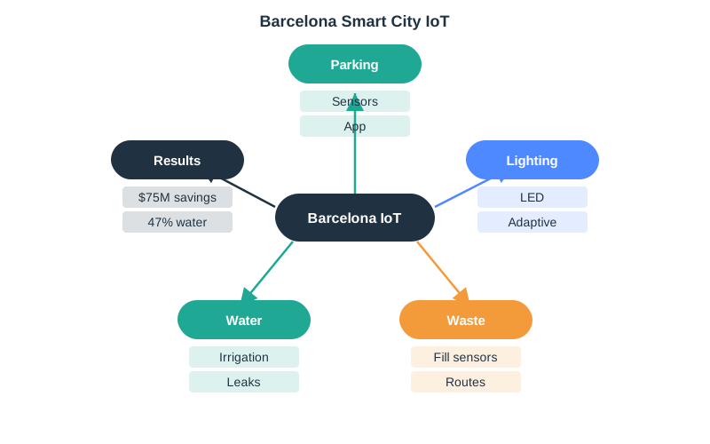
Read the Barcelona and Volkswagen cases as evidence chains rather than success stories. The case evidence starts with a field condition, such as parking occupancy or robot vibration, then follows the path through sensing, communication, edge processing, workflow integration, user adoption, and measured operating result. A deployment lesson is transferable only when that whole chain is visible. Otherwise a team may copy the most visible technology, such as LoRaWAN, edge gateways, or a dashboard, while missing the calibration, maintenance, trust-building, and integration work that made the deployment useful.
That framing also separates local context from reusable pattern. Barcelona’s service mix, public procurement, and municipal data-sharing constraints are city-specific; Volkswagen’s robot fleet, production takt time, and maintenance culture are factory-specific. The reusable pattern is the disciplined loop: define the operating decision, instrument the right point, preserve uncertainty, connect the result to work, and measure whether people actually change behavior.
26.5 The Cross-Detection Problem
Because the magnetometer measures a field, not a boundary, a large vehicle in an adjacent bay can distort the field enough to look like an occupant, creating a false positive that tells drivers a free bay is taken. This cross-detection is the defining real-world challenge of magnetic parking sensors, and it is solved by calibration, not by a bigger sensor.
Each sensor learns its own empty-bay baseline field and flags occupancy only when the local change exceeds a threshold set above the crosstalk a neighbour’s car produces. The direct occupant shifts the field by a large amount, several microtesla or more close up. A neighbour’s car produces a smaller shift that the threshold rejects.
| Source | Field change at sensor | Decision |
|---|---|---|
| Empty bay | Roughly baseline, for example 50 microtesla | Vacant |
| Car in this bay | Large local shift | Occupied |
| Car in adjacent bay | Small shift, or crosstalk | Reject, below threshold |
Worked example. A sensor calibrated to a 50 microtesla baseline sees a 12 microtesla swing when a car parks directly over it, but only a 3 microtesla swing from a truck in the next bay. Setting the occupancy threshold at 6 microtesla catches the real occupant and rejects the neighbour. Where bays are tight or vehicles huge, a single magnetometer’s margin shrinks, and designs add a second sensing mode, such as radar, or fuse two axes of the magnetic reading to separate “above me” from “beside me.”
For practitioners, the case-study question is what must be recorded before rollout expands. Parking sensors need installation depth, bay geometry, empty-baseline sample, adjacent-vehicle test result, firmware version, LoRaWAN spreading factor, gateway RSSI/SNR, battery estimate, and complaint history. Volkswagen’s maintenance case needs the same discipline in a factory form: robot asset id, sensor placement, model version, confidence threshold, technician acknowledgement, work-order outcome, and false-positive review. Those records let teams tune thresholds without guessing and separate a weak sensor, weak model, weak network, or weak workflow.
26.6 Event Reporting Failure Mode
To reach a 5-10 year battery life on LoRaWAN, the sensor reports on state change, not periodically: it sends a message only when a bay transitions between vacant and occupied. This slashes airtime because a bay may change a few times a day, and it respects the EU 868 MHz 1% duty-cycle limit and LoRaWAN’s tiny data budget. But event-driven reporting has a specific failure mode: LoRaWAN uplinks are unconfirmed and can be lost, and if the single “now occupied” message is dropped, the app shows the bay free indefinitely. The state is stuck until the next change.
The engineering answer is a periodic heartbeat: alongside change events, the sensor sends its current state on a slow schedule, such as every few hours, so a lost transition self-corrects at the next heartbeat, and the server can also detect a dead sensor by its silence. This is the classic event-driven trade-off: events give efficiency, heartbeats give recoverability. Getting the balance right is what makes the deployment trustworthy rather than merely cheap.
Worked example. A car leaves a bay and the sensor’s “vacant” uplink is lost to interference. With pure event reporting the app wrongly shows the bay occupied for hours, sending drivers past an empty space. Add a 4-hour heartbeat and the true vacant state is restored at the next beat, bounding the error to at most one heartbeat interval. The same heartbeat lets the backend flag a sensor that has gone silent for a day as failed. The transferable decision from this case, pairing change-events with a recovery heartbeat, applies to any lossy, low-power, event-driven IoT link.
Under the hood, the backend should treat every parking or maintenance event as a state update with evidence attached. A parking message should include device id, bay id, sequence number, measured field delta, threshold version, battery, RSSI/SNR, gateway id, event timestamp, and whether the message is a change event or heartbeat. A maintenance alert should carry the sensor window, feature vector version, model id, confidence, asset state, and work-order link. That metadata is what lets operators reconcile stale app state, missed messages, and ignored alerts after the fact.