33  GPS and Outdoor Positioning

33.1 Start Simple

Outdoor positioning begins with a simple question: can the receiver see enough sky to support the promise? Start with satellite geometry, timing error, multipath, update rate, and power, then decide what the user should see when the fix is good, degraded, or unavailable.

Phoebe’s Field Notes: Why the Pseudorange Needs a Fourth Satellite

Phoebe’s Why

Time-of-flight is simple physics – distance is speed times time – but GPS turns that simple idea into a genuinely hard problem the instant you admit the receiver’s own clock is not trustworthy. A cheap crystal oscillator can drift by microseconds, and at the speed of light a microsecond of timing error is a football field of position error. So every range GPS measures is really a “pseudorange”: the true geometric distance to a satellite plus one shared unknown, the receiver’s clock bias, riding on every single measurement. That is not a nuisance to filter out – it is the reason a GPS fix needs a fourth satellite that has nothing to do with three-dimensional space.

The Derivation

Time-of-flight distance:

\[d = c\,\Delta t\]

Each satellite \(i\) gives a pseudorange \(\rho_i\) that mixes the true range to the (known) satellite position with the (unknown) receiver clock bias \(b\):

\[\rho_i = c\,(t_{rx}-t_{tx,i}) = \sqrt{(x-x_i)^2+(y-y_i)^2+(z-z_i)^2} + c\,b\]

Four unknowns – receiver position \((x,y,z)\) and clock bias \(b\) – need four independent equations, i.e. four satellites, before the system is solvable; a fifth satellite and beyond turns it into the overdetermined least-squares fix this chapter already describes.

Worked Numbers: This Chapter’s Own Timing Numbers

• Time of flight from a satellite at this chapter’s own \(20{,}200\) km altitude: \(t=20{,}200{,}000/299{,}792{,}458=0.0674\) s \(=67.4\) ms – matching the “67-68 milliseconds” the interactive above already shows.
• \(1\ \mu\text{s}\) clock error \(\to\) range error \(=299{,}792{,}458\times10^{-6}=299.8\) m \(\approx300\) m, exactly this chapter’s own figure.
• To hold position error to \(3.00\) m, the pseudorange timing needs precision \(\Delta t=3.00/299{,}792{,}458=1.00\times10^{-8}\) s \(=10.0\) ns – about 100 times tighter than the 1 microsecond that already costs 300 m.
• This chapter’s “~1 nanosecond/day” atomic-clock stability translates to a range creep of \(299{,}792{,}458\times10^{-9}=0.300\) m per day if left uncorrected – small per day, but why the ground segment still uploads clock corrections on a schedule rather than trusting the onboard oscillator indefinitely.

33.2 Summary

GPS/GNSS positioning depends on satellite timing, pseudoranges, geometry, receiver clocks, and environmental multipath. Outdoor positioning designs should account for accuracy limits, power use, update rate, and failure conditions.

Chapter Roadmap

This chapter moves from product promise to GPS math and field validation.

1. First you separate the outdoor location promise from the receiver’s searching, stale, good, and degraded states.
2. Then you connect time-of-flight, pseudoranges, and the four-satellite clock-offset problem.
3. Next you inspect synchronization, relativity, multipath, and satellite geometry as real error sources.
4. Finally you use quizzes and field exercises to decide when the fix is good enough to act on.

Checkpoint callouts mark the main stops; deep calculation panels can be revisited after the first read.

In 60 Seconds

GPS determines position by measuring time-of-flight from at least 4 satellites, solving for 3D position plus clock offset. Signals travel at the speed of light, making timing critical – a 1 microsecond clock error equals 300 meters of position error, which is why satellites carry atomic clocks. The multipath problem (signals bouncing off buildings) is GPS’s biggest challenge in urban environments, degrading accuracy from 5-10 meters to 50+ meters.

33.3 Learning Objectives

By the end of this chapter, you will be able to:

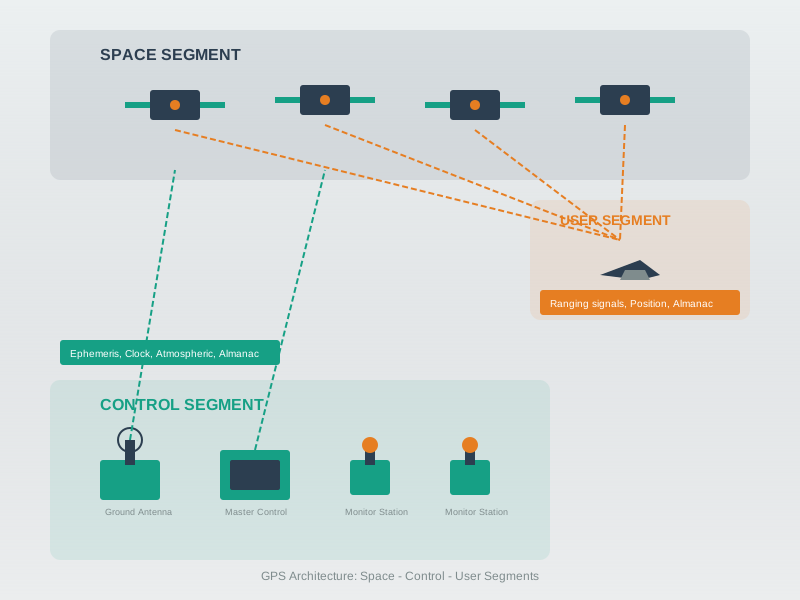
• Explain GPS/GNSS Architecture: Describe the space, control, and user segments of satellite navigation systems
• Calculate Positioning from Satellites: Apply Time of Flight and TDoA principles to determine position
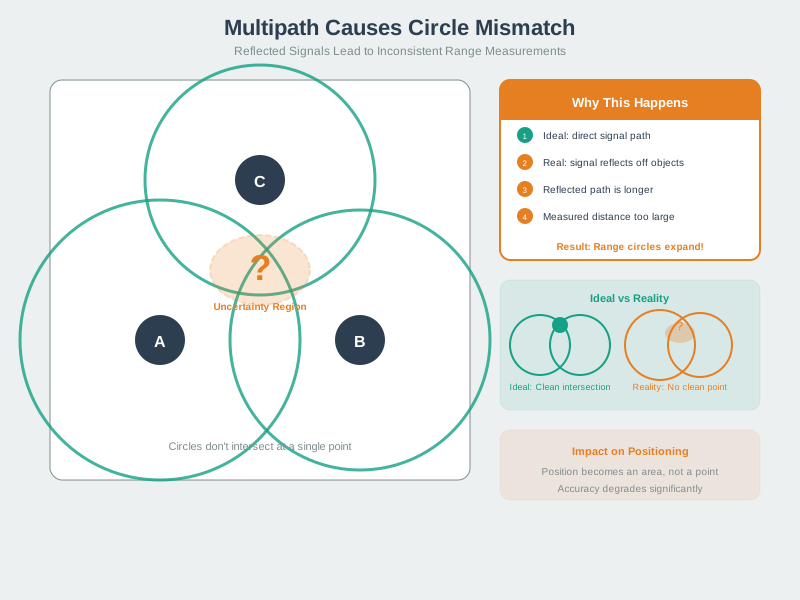
• Diagnose Multipath Effects: Distinguish how signal reflections degrade positioning accuracy in different environments
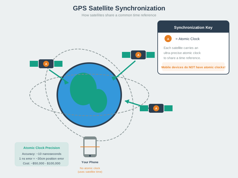
• Justify Clock Synchronization: Explain why atomic clocks are essential and demonstrate how pseudoranges compensate for receiver clock errors

GPS and Outdoor Positioning

GPS (Global Positioning System) works by measuring the time it takes for radio signals to travel from satellites to your device. With signals from at least 4 satellites, a receiver can calculate its 3D position. The math is elegant but the engineering is challenging: signals travel at the speed of light, so a 1 microsecond clock error means 300 meters of position error – which is why satellites carry atomic clocks. The biggest real-world challenge is multipath – signals bouncing off buildings in cities can degrade accuracy from 5 meters to 50+ meters.

Key Concepts

• GPS: Global Positioning System providing 3-10 metre outdoor accuracy using triangulation from 4+ satellites, consuming 20-100 mA active current.
• Indoor Positioning: Techniques (BLE beacons, UWB, Wi-Fi RSSI, IMU dead-reckoning) achieving 0.1-5 metre accuracy where GPS signals are unavailable.
• Geofencing: Virtual geographic boundary triggering automated actions when a tracked asset enters or exits the defined area.
• Dead Reckoning: Position estimation using last known location plus measured movement (speed, heading) when GPS signal is lost.
• RSSI-Based Positioning: Location estimation from signal strength of known beacon nodes, achieving 2-5 metre accuracy in calibrated environments.
• Ultra-Wideband (UWB): Radio technology providing 10-30 cm indoor positioning accuracy using time-of-flight measurements between anchor nodes.
• Location Privacy: User right to control who can access their location history and how granular that location data is stored.

33.4 Prerequisites

• Location Awareness Fundamentals: Understanding of positioning technology landscape

33.5 GPS Timing as Product Context

GPS/GNSS is not just a map dot. It is a timing system that lets an IoT product infer outdoor context from weak satellite signals, known orbits, receiver clock error, and a changing view of the sky. The product decision is what the system should do with that context: show a vehicle route, confirm a gate arrival, enforce a geofence, steer a machine, timestamp a field event, or refuse an unsafe automation.

Good outdoor location design starts by separating the fix lifecycle from the user promise. A receiver may be searching, downloading assistance data, using a two-dimensional fix, using a three-dimensional fix, coasting on dead reckoning, or reporting a stale position after losing sky view. The interface should not show all of those states as the same precise blue dot.

That distinction matters because the same receiver can be excellent in one context and misleading in another. A field sensor with a clear antenna view may produce stable fixes every few minutes. A courier phone in an urban canyon may report plausible but wrong locations because reflected signals make pseudoranges too long. A tracker under a vehicle dashboard may acquire slowly because metal and glass attenuate the satellite signals. The product should expose the quality difference before it triggers an action.

Design the user promise around the consequence. “The asset was last seen near gate 4 at 10:31” is a different promise from “unlock the gate because the vehicle is here.” A route display can tolerate a snapped-to-road correction, but an audit trail should keep the raw fix and the corrected point separate. A safety geofence should require dwell time, accuracy radius, and current timestamp instead of accepting a stale point inside the boundary.

• Acquisition: cold start, warm start, assisted GPS, and time-to-first-fix affect what a user sees during setup and recovery.
• Continuity: update rate, power mode, antenna placement, map matching, and IMU handoff decide whether tracks are smooth or jumpy.
• Trust: accuracy radius, timestamp, fix type, and fallback wording tell users when the location is useful enough to act on.

33.6 Receiver State Machine Design

Treat the GNSS receiver as a stateful component. During setup, record whether the device has a valid time source, recent almanac, recent ephemeris, enough satellites, acceptable HDOP, and a clear antenna view. During operation, record whether the receiver is using GPS alone or a multi-GNSS fix with Galileo, GLONASS, BeiDou, or QZSS; whether position comes from GNSS, Android Fused Location Provider, Apple Core Location, or an external receiver; and whether the product has applied map matching or sensor fusion.

For battery IoT devices, the correct update rate is rarely “as fast as possible.” A livestock collar, rental scooter, delivery app, and safety beacon have different duty cycles. Track the cost of each fix in active current, radio upload, cloud storage, and user attention. Use batching, geofence triggers, adaptive sampling, and motion detection when continuous GNSS would waste energy without improving the decision.

Build acceptance tests around the places where GNSS changes behavior. Test open-sky startup, tree cover, urban street canyons, indoor-to-outdoor transition, pocket or bag carry, low battery, airplane mode, poor antenna orientation, and recovery after several hours powered off. For embedded modules, include antenna ground plane, enclosure material, cable length, and placement near radios or processors. For phones, include permission denial, approximate-location mode, background throttling, and operating-system power saving.

Use different display and automation rules for different fix classes. A dashboard can show a stale position with a timestamp and grey styling. A dispatch workflow can route a driver only after speed, heading, and map-matched road segment agree. A custody workflow can ask for a QR or NFC confirmation at the site when the GNSS radius is larger than the loading bay. Those rules make uncertainty operational instead of leaving support staff to explain why a blue dot looked exact.

1. Specify the fix policy: define no-fix, searching, coarse, good, stale, and degraded states with display text and allowed automations.
2. Specify the movement policy: combine speed, heading, accelerometer, gyroscope, odometer, or map-matched road segment only when their timing and frames line up.
3. Specify the power policy: choose continuous tracking, periodic fixes, event-triggered fixes, or user-requested fixes based on consequence and battery life.

33.7 Under the Hood: The Fix Is a Pipeline

A practical GNSS pipeline starts with RF acquisition and ends with a position, velocity, and time solution. The receiver searches for signals such as GPS L1 C/A, GPS L5, Galileo E1/E5, BeiDou B1/B2, or GLONASS signals; locks code phase and Doppler; decodes navigation data; applies ephemeris, clock, atmospheric, and relativistic corrections; estimates pseudoranges; and solves for receiver position and clock offset. Many modules expose the result through NMEA sentences such as GGA, RMC, GSA, and GSV, or through binary protocols such as UBX.

The product should keep the quality fields near the coordinate. Useful fields include fix type, HDOP/VDOP/PDOP, satellite count, constellation mix, C/N0 signal quality, estimated horizontal error, estimated vertical error, speed, course over ground, timestamp, leap-second/time status, assistance-data age, and antenna status. If a cloud service or map layer changes the coordinate, keep both the raw fix and the processed position so operations teams can distinguish receiver behavior from product logic.

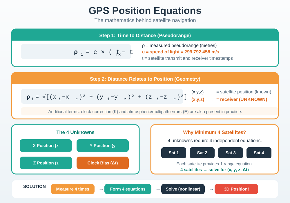
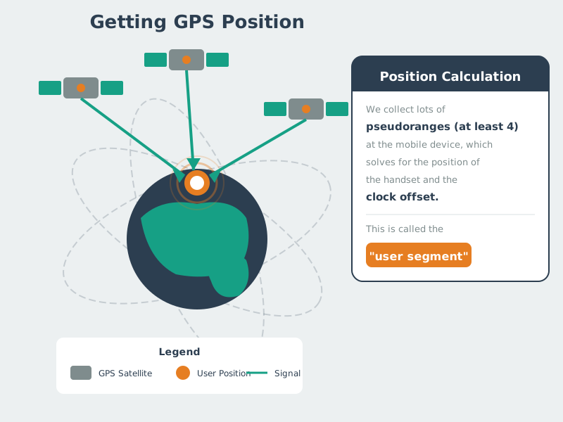
The receiver clock is the reason GPS needs at least four satellites for a full fix. Each satellite gives one pseudorange equation. The unknowns are receiver x, y, z, and receiver clock offset from GNSS time. Once more than four satellites are available, the solver can use an overdetermined least-squares solution and report dilution-of-precision values that describe the geometry. Good geometry does not remove all error, but poor geometry can make otherwise valid measurements produce a weak position.

Assistance and correction services change the pipeline. Assisted GNSS can provide approximate time, approximate location, almanac, or ephemeris data over a network to reduce time-to-first-fix. SBAS, DGPS, RTK, or PPP can reduce some satellite, clock, and atmospheric errors when the receiver and service support them. Those features should be represented in product metadata because a centimeter-capable RTK rover in fixed mode is making a different claim from a phone-grade coarse fix.

• Cold-start risk: without valid time, location, almanac, or ephemeris, first fix can be slow; assisted data over SUPL or a vendor service changes startup behavior.
• Urban risk: multipath and blocked sky can pass through the solver as plausible coordinates; map matching and inertial smoothing help but can also hide real uncertainty.
• System risk: a geofence, route, or safety command should consume the quality-aware location event, not a naked latitude/longitude pair.

Checkpoint: Fix Lifecycle

You now know:

• A GPS product should show searching, stale, degraded, and good fixes differently.
• The useful event includes fix type, quality fields, timestamp, source, and fallback wording.
• Power policy and automation policy should follow consequence, not raw latitude and longitude.

With the product states named, the next question is where the numbers behind a GPS fix come from.

33.8 Global Navigation Satellite Systems

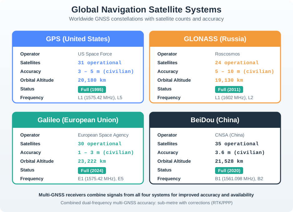
Figure 33.1: Diagram showing GNSS systems worldwide with satellite counts and accuracy specifications.

GPS (Global Positioning System): The first and most widely deployed Global Navigation Satellite System (GNSS), which has come to dominate outdoor positioning.

To understand GPS fully, we first examine two important techniques…

33.9 Time of Flight (ToF)

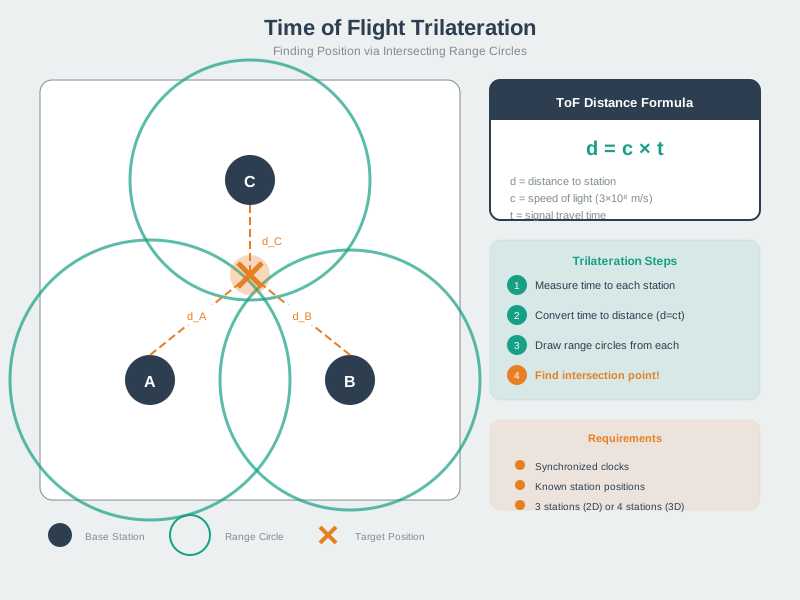
Time of Flight: Measure the time taken for a signal to propagate from transmitter to receiver.

Figure 33.2: Time of Flight Concept

Distance Calculation:

Distance = Speed of Light × Time of Flight
d = c × Δt

where:
- c = 299,792,458 m/s (speed of light in vacuum)
- Δt = reception time - transmission time

Time of Flight to Distance

viewof tof_time_ms = Inputs.range([0, 100], {
  value: 67.33,
  step: 0.01,
  label: "Signal Travel Time (ms)"
})

viewof tof_speed_of_light = Inputs.select(
  [299792.458, 299792, 300000],
  {
    value: 299792.458,
    label: "Speed of Light (km/s)",
    format: x => x === 299792.458 ? "Exact (299,792.458)" : x === 299792 ? "Approx (299,792)" : "Rounded (300,000)"
  }
)

tof_distance_km = (tof_time_ms / 1000) * tof_speed_of_light

html`<div style="padding: 12px; background: #f8f9fa; border-left: 4px solid #16A085; margin: 12px 0;">
  <strong style="color: #2C3E50;">Distance:</strong>
  <span style="color: #E67E22; font-size: 1.2em; font-weight: bold;">${tof_distance_km.toFixed(2)} km</span>
  <span style="color: #7F8C8D; margin-left: 8px;">(${(tof_distance_km * 1000).toFixed(0)} meters)</span>
</div>`

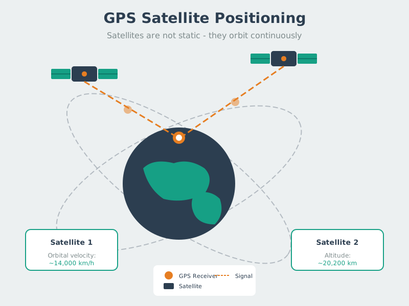
Try it: Adjust the signal travel time to see how distance changes. GPS satellites orbit at ~20,200 km altitude, so typical travel times are 67-68 milliseconds.

Critical Challenge: Both transmitter and receiver must have synchronized clocks to know the true transmission time.

Clock Error Impact

viewof clock_error_value = Inputs.range([0, 1000], {
  value: 1,
  step: 0.1,
  label: "Clock Error Value"
})

viewof clock_error_unit = Inputs.select(
  ["nanoseconds", "microseconds", "milliseconds"],
  {
    value: "microseconds",
    label: "Time Unit"
  }
)

clock_error_seconds = clock_error_unit === "nanoseconds" ? clock_error_value * 1e-9 :
                      clock_error_unit === "microseconds" ? clock_error_value * 1e-6 :
                      clock_error_value * 1e-3

position_error_meters = clock_error_seconds * 299792458

html`<div style="padding: 12px; background: #fff3cd; border-left: 4px solid #E67E22; margin: 12px 0;">
  <strong style="color: #2C3E50;">Position Error:</strong>
  <span style="color: #E74C3C; font-size: 1.2em; font-weight: bold;">${position_error_meters.toFixed(2)} meters</span>
  ${position_error_meters > 1000 ? `<span style="color: #7F8C8D; margin-left: 8px;">(${(position_error_meters / 1000).toFixed(2)} km)</span>` : ''}
  <div style="margin-top: 8px; color: #7F8C8D; font-size: 0.9em;">
    This is why GPS satellites need atomic clocks with ~1 nanosecond/day accuracy!
  </div>
</div>`

Key insight: Even tiny clock errors create huge position errors because signals travel at light speed (300 million meters/second).

33.10 The Multipath Problem

Figure 33.3: Multipath problem in GPS

Multipath: Signals reflect off objects, creating multiple paths between transmitter and receiver.

Impact:

• Fine for communications: Multiple signals can be combined
• Kills positioning: Makes distances appear longer than reality
• Indoor environments: Severe multipath due to many reflective surfaces

Checkpoint: Timing and Reflections

You now know:

• Time-of-flight turns signal travel time into distance, so 67-68 ms maps to GPS-orbit ranges.
• A 1 microsecond clock error means about 300 m of range error.
• Multipath can move an urban fix from 5-10 m accuracy to 50+ m error.

33.11 Time Difference of Arrival (TDoA)

Figure 33.4: Time difference of arrival

The Problem with Simple ToF:

• Mobile device and fixed sites separated by large distances
• Cannot keep clocks synchronized
• RF signals travel at c, so 1 μs sync error = 300m position error

TDoA Solution:

• Accept that clocks aren’t synced
• Solve for the clock offset as an additional unknown
• Any single range is wrong, but every range is wrong by the same amount
• These erroneous ranges are called pseudoranges

Key Requirements for TDoA:

1. Base Stations Must Be Synchronized:
   • Lay cables between stations
   • Use GPS (ironically!)
   • Give them all atomic clocks ($$$)
2. Mobile Device Clock Can Be Wrong:
   • Clock offset becomes an additional unknown to solve
   • Need N+1 stations for N-dimensional positioning
   • 3D position + clock offset = 4 unknowns → need 4 satellites

GPS uses the same idea in reverse: the expensive clocks are in space, and the receiver solves its own cheap clock error as part of the position.

33.12 GPS Architecture

Figure 33.5: GPS System Overview

GPS is TDoA (Inverted):

• Satellites play the part of static devices (but are transmitters)
• Mobile device measures reception time using its clock
• Uses satellite’s transmitted time for the time difference
• For each satellite: measures (ToF + c × clockOffset)
• These are pseudoranges (erroneous distances)

33.13 Satellite Synchronization

Figure 33.6: How are satellites synced

How Satellites Stay Synchronized:

1. Atomic Clocks On Board (Caesium or Rubidium)
   • Cost: ~$100,000 per clock
   • Accuracy: ~1 nanosecond per day
   • All satellites share time reference
2. But They Aren’t Static?
   • True! But we know their orbits precisely
   • Can predict positions quite accurately
   • Small errors do creep in…
3. Ground Control Segment:
   • Dedicated ground stations monitor satellite orbits
   • Track actual positions vs predicted
   • Upload corrections to satellites
   • Must model relativistic effects!

Figure 33.7: Satellite Orbit Monitoring

Relativistic Effects:

• Special Relativity: Satellite clocks run slower due to velocity (~7 μs/day slower)
• General Relativity: Satellite clocks run faster due to weaker gravity (~45 μs/day faster)
• Net Effect: ~38 μs/day faster → must be corrected!

Relativity Effects in GPS

Without relativistic corrections, GPS would accumulate ~10 km of error per day. Here’s why:

Special Relativity (time dilation from velocity): Satellites orbit at \(v \approx 3,874\) m/s. Time dilation factor: \[\gamma = \frac{1}{\sqrt{1 - \frac{v^2}{c^2}}} \approx 1 + \frac{v^2}{2c^2}\]

For GPS: \(\frac{v^2}{2c^2} = \frac{(3,874)^2}{2 \times (3 \times 10^8)^2} \approx 8.3 \times 10^{-11}\)

Clock runs slower by: \(8.3 \times 10^{-11} \times 86,400 \text{ s/day} \approx 7.2\) μs/day

General Relativity (gravitational time dilation): At GPS orbit altitude (20,200 km), gravitational potential is weaker than at Earth’s surface. Clock rate difference: \[\frac{\Delta t}{t} = \frac{GM}{c^2} \left(\frac{1}{r_{\text{surface}}} - \frac{1}{r_{\text{orbit}}}\right)\]

Where \(GM_{\text{Earth}} = 3.986 \times 10^{14}\) m³/s², \(r_{\text{surface}} = 6.37 \times 10^6\) m, \(r_{\text{orbit}} = 2.66 \times 10^7\) m.

\[\frac{\Delta t}{t} \approx 5.3 \times 10^{-10} \Rightarrow 5.3 \times 10^{-10} \times 86,400 \approx 45.9 \text{ μs/day faster}\]

Net effect: \(45.9 - 7.2 = 38.7\) μs/day clock advancement

Position error if uncorrected: Light travels at \(c = 3 \times 10^8\) m/s, so: \[\text{Error} = c \times \Delta t = 3 \times 10^8 \times 38.7 \times 10^{-6} \approx 11,600 \text{ m/day}\]

GPS solution: Satellite clocks are pre-adjusted to run at 10.22999999543 MHz (instead of exactly 10.23 MHz) to cancel the net +38.7 μs/day drift.

Relativistic Time Dilation

viewof relativity_velocity = Inputs.range([1000, 8000], {
  value: 3874,
  step: 10,
  label: "Satellite Velocity (m/s)"
})

viewof relativity_altitude = Inputs.range([10000, 30000], {
  value: 20200,
  step: 100,
  label: "Orbit Altitude (km)"
})

// Constants
c_light = 299792458  // m/s
GM_earth = 3.986e14  // m³/s²
r_surface = 6.37e6   // meters
seconds_per_day = 86400

// Special relativity (time dilation from velocity)
v_squared_over_2c_squared = (relativity_velocity * relativity_velocity) / (2 * c_light * c_light)
special_relativity_us_per_day = v_squared_over_2c_squared * seconds_per_day * 1e6

// General relativity (gravitational time dilation)
r_orbit = (relativity_altitude * 1000) + r_surface
delta_t_over_t = (GM_earth / (c_light * c_light)) * ((1 / r_surface) - (1 / r_orbit))
general_relativity_us_per_day = delta_t_over_t * seconds_per_day * 1e6

// Net effect
net_effect_us_per_day = general_relativity_us_per_day - special_relativity_us_per_day

// Position error per day if uncorrected
position_error_per_day = (net_effect_us_per_day * 1e-6) * c_light

html`<div style="padding: 16px; background: #f8f9fa; border: 1px solid #dee2e6; border-radius: 4px; margin: 12px 0;">
  <div style="display: grid; grid-template-columns: 1fr 1fr; gap: 12px; margin-bottom: 12px;">
    <div style="padding: 8px; background: #e3f2fd; border-radius: 4px;">
      <div style="color: #2C3E50; font-size: 0.9em;">Special Relativity (slower)</div>
      <div style="color: #3498DB; font-size: 1.1em; font-weight: bold;">-${special_relativity_us_per_day.toFixed(1)} μs/day</div>
    </div>
    <div style="padding: 8px; background: #f3e5f5; border-radius: 4px;">
      <div style="color: #2C3E50; font-size: 0.9em;">General Relativity (faster)</div>
      <div style="color: #9B59B6; font-size: 1.1em; font-weight: bold;">+${general_relativity_us_per_day.toFixed(1)} μs/day</div>
    </div>
  </div>
  <div style="padding: 12px; background: ${net_effect_us_per_day > 0 ? '#fff3cd' : '#d1ecf1'}; border-left: 4px solid ${net_effect_us_per_day > 0 ? '#E67E22' : '#16A085'}; border-radius: 4px;">
    <strong style="color: #2C3E50;">Net Effect:</strong>
    <span style="color: #E67E22; font-size: 1.2em; font-weight: bold;">${net_effect_us_per_day > 0 ? '+' : ''}${net_effect_us_per_day.toFixed(1)} μs/day</span>
    <div style="margin-top: 8px; color: #2C3E50;">
      <strong>Uncorrected Position Error:</strong>
      <span style="color: #E74C3C; font-weight: bold;">${(position_error_per_day / 1000).toFixed(1)} km/day</span>
      <span style="color: #7F8C8D; margin-left: 4px;">(${position_error_per_day.toFixed(0)} meters)</span>
    </div>
  </div>
</div>`

Explore: Change the satellite velocity or altitude to see how relativistic effects change. GPS satellites at 20,200 km altitude traveling at 3,874 m/s experience a net +38.7 μs/day clock advancement, which must be corrected.

Checkpoint: Satellite Timekeeping

You now know:

• Satellite atomic clocks and ground control keep the shared time reference usable.
• Relativity matters at GPS orbit: about 7 us/day slower from velocity, 45 us/day faster from gravity, and 38.7 us/day net.
• Without correction, the timing drift would accumulate about 10 km of position error per day.

33.14 GPS Position Calculation

Figure 33.8: GPS position calculation

Position Equations:

For each satellite \(i\):

\[ \rho_i = \sqrt{(x_i - x_r)^2 + (y_i - y_r)^2 + (z_i - z_r)^2} + c \cdot \Delta t + E_i \]

Where: - \(\rho_i\) = pseudorange to satellite \(i\) (measured) - \((x_i, y_i, z_i)\) = satellite \(i\) position (known from ephemeris) - \((x_r, y_r, z_r)\) = receiver position (unknown) - \(c\) = speed of light - \(\Delta t\) = receiver clock offset (unknown) - \(E_i\) = error term (atmospheric delays, etc.)

Four Unknowns:

1. \(x_r\) (receiver X position)
2. \(y_r\) (receiver Y position)
3. \(z_r\) (receiver Z position)
4. \(\Delta t\) (clock offset)

Need at least 4 satellites to solve for 4 unknowns!

33.15 Position from Satellite Signals

Scenario: Your GPS receiver picks up signals from 4 satellites. You need to understand how position is derived from raw timing measurements.

Given data (simplified to 2D for clarity):

Satellite	Known Position (km)	Signal Travel Time	Pseudorange (km)
Sat A	(0, 20200)	67.33 ms	20,185.0
Sat B	(14290, 14290)	67.28 ms	20,170.0
Sat C	(-14290, 14290)	67.38 ms	20,200.0
Sat D	(20200, 0)	67.40 ms	20,206.0

Step 1: Convert time to distance

Each pseudorange = speed of light x travel time:

• Sat A: 299,792 km/s x 0.06733 s = 20,185.0 km

Step 2: Notice the clock offset

All pseudoranges include the same unknown clock error. If the receiver clock is 50 nanoseconds fast, every pseudorange is 15 meters too long. The fourth satellite lets us solve for this offset.

Step 3: Solve the system of equations

With 4 equations and 4 unknowns (x, y, z, clock offset), the receiver’s least-squares solver finds the position. In practice, modern receivers process signals from 10-12 satellites simultaneously, using the extras to improve accuracy and detect anomalies.

Key insight: Each additional satellite beyond 4 reduces position error by approximately 20-30%. A receiver tracking 8 satellites achieves roughly 2-3 meter accuracy versus 5-10 meters with exactly 4.

33.16 Uber GPS Accuracy in Manhattan

Uber discovered in 2015 that GPS-based pickup locations in Manhattan were consistently wrong by 20-50 meters – enough to place riders on the wrong side of a city block or on a different street entirely. This caused 15-20% of Manhattan pickups to require phone calls between driver and rider, adding an average 4.2 minutes per trip and costing an estimated $50 million annually in driver idle time.

Root cause analysis: Manhattan’s dense skyscraper grid created severe multipath interference. GPS signals bounced off glass and steel facades, arriving at smartphone receivers via indirect paths that added 50-200 nanoseconds of delay – translating to 15-60 meters of position error.

The technical challenge in numbers:

Environment	GPS Accuracy	Pickup Success Rate
Open suburban	3-5 meters	94%
Low-rise urban	8-15 meters	87%
Midtown Manhattan	20-50 meters	72%
Financial District (canyon)	30-80 meters	61%

Uber’s multi-technology solution (2016-2019):

1. Sensor fusion: Combined GPS with phone accelerometer and gyroscope data. Dead reckoning between GPS fixes reduced error during multipath events.
2. Map matching: Snapped estimated positions to the road network using Hidden Markov Models. A rider on 5th Avenue would never be placed in the middle of a building.
3. 3D building models: Used Manhattan building height data to predict which satellites would have clear sky views versus multipath interference, weighting satellite signals accordingly.
4. Wi-Fi fingerprinting: Added Wi-Fi access point signal strengths as supplementary positioning data in areas with dense AP coverage.

Results after implementation:

• Manhattan pickup accuracy improved from 25-50m median error to 8-12m
• Phone calls for pickup coordination dropped 62%
• Average pickup time decreased by 2.8 minutes
• Annual savings estimated at $32 million in reduced driver idle time

Lesson for IoT designers: Any IoT application that depends on GPS positioning in urban environments must budget for multipath mitigation. Raw GPS alone is insufficient – sensor fusion, map matching, and supplementary positioning technologies are essential for sub-10-meter accuracy in built-up areas.

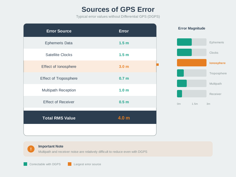
33.17 GPS Error Sources

Figure 33.9: GPS error sources

Signal Strength Challenge:

• GPS signal transmitted at 20 watts
• Travels 20,200 km (GPS orbit altitude)
• Received power: ~10^-16 watts (incredibly weak!)
• Various atmospheric effects introduce errors

Error Source	Typical Error	Mitigation
Ionospheric delay	±5 m	Dual-frequency correction
Tropospheric delay	±0.5 m	Modeling
Satellite clock	±2 m	Ground station corrections
Ephemeris	±2.5 m	Frequent updates
Multipath	±1 m	Antenna design, averaging
Receiver noise	±0.3 m	Better receivers

Checkpoint: Operational Accuracy

You now know:

• Four satellites solve the minimum four unknowns; 10-12 satellites let receivers improve and cross-check the solution.
• Dense streets can add 50-200 ns of delay and 15-60 m of position error.
• A weak 20 W satellite signal arriving from 20,200 km needs correction, filtering, and honest quality metadata.

33.18 Knowledge Check

Quiz: GPS Fundamentals

Interactive Quiz: Match Concepts

Interactive Quiz: Sequence the Steps

Key Takeaway

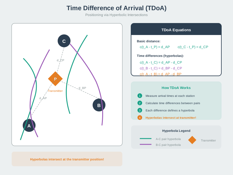
GPS is an inverted TDoA system where satellites broadcast synchronized time signals and receivers calculate position from pseudoranges. Four satellites are the minimum (3 position unknowns + 1 clock offset), but more satellites improve accuracy through overdetermined solutions. The system’s genius is treating the receiver’s cheap clock offset as a solvable unknown rather than requiring expensive atomic clocks in every device. The biggest practical limitations are multipath (signal reflections in cities) and the complete inability to work indoors due to signal attenuation through building materials.

For Kids: Meet the Sensor Squad!

GPS is like playing Marco Polo with satellites in SPACE!

33.18.1 Messages from Space

“How does my phone know where I am?” asked Lila the LED one day, staring at the blue dot on a map.

Sammy the Sensor knew the answer. “There are 24 special satellites orbiting Earth, way up in space – about 20,000 kilometers high! Each one is basically shouting ‘I’M HERE and the time is 3:00:00.000000!’”

“But how does that help?” asked Lila.

“Imagine you’re blindfolded in a big park,” said Max the Microcontroller. “Three friends stand in different spots and each one shouts ‘I’m 50 meters from you!’ or ‘I’m 30 meters from you!’ With three distances, there’s only ONE spot where you could be standing!”

“That’s TRILATERATION!” cheered Bella the Battery. “GPS works the same way, but instead of friends shouting, it’s satellites sending time signals. Your phone calculates how far each satellite signal traveled by how long it took to arrive.”

“But here’s the tricky part,” said Sammy. “Radio signals travel at the SPEED OF LIGHT – 300,000 kilometers per second! That’s SO fast that if your phone’s clock is off by just ONE MILLIONTH of a second, it’s wrong by 300 meters!”

“That’s why we need a FOURTH satellite!” explained Max. “Three satellites tell us where we are, and the fourth one helps us figure out exactly what time it is. The satellites have super-expensive atomic clocks that cost $100,000 each, but our phones can figure out the right time by using math!”

“So GPS is really about TIME, not just PLACE!” realized Lila.

“Exactly! And the satellites are so far away that their signals are incredibly weak when they reach us. That’s why GPS doesn’t work inside buildings – the signals can’t get through walls and ceilings!”

33.18.2 Key Words for Kids

Word	What It Means
Satellite	A special machine orbiting Earth in space that sends time signals to GPS receivers
Speed of Light	The fastest speed in the universe – 300,000 km per second! GPS signals travel this fast
Atomic Clock	A super-accurate clock on satellites that loses less than 1 second in a MILLION years
Pseudorange	A distance measurement that’s slightly wrong because your phone’s clock isn’t perfect

Concept Relationships

How this chapter connects to other IoT concepts:

• Foundation for: GPS Accuracy Enhancement builds on error sources and pseudorange concepts to implement DGPS/RTK corrections
• Contrasts with: Indoor Positioning which requires entirely different technologies where satellite signals fail
• Atomic clocks: Satellite Synchronization explains why GPS provides an authoritative time source for distributed IoT systems
• Multipath: Wireless Fading and Interference explains why signal reflection affects all RF systems, not just GPS
• Case study: Urban IoT Challenges Manhattan multipath problem affects all outdoor location services

See Also

Related topics for deeper exploration:

• GNSS Constellations: Details on GLONASS, Galileo, and BeiDou systems that supplement GPS
• Relativistic Effects on Satellites: Why satellite clocks run 38 microseconds fast per day due to gravity and velocity
• GPS Error Sources: How ionospheric delay, tropospheric delay, multipath, and receiver noise affect GPS accuracy
• Kalman Filtering for GPS: Mathematical framework for combining GPS with IMU dead reckoning
• A-GPS and Assistance Data: How cellular networks accelerate GPS acquisition via ephemeris assistance

Try It Yourself

The exercises turn the same quality fields into field evidence: satellite geometry, acquisition time, multipath, and track smoothness.

Hands-on exercises to understand GPS mechanics:

33.18.3 Exercise 1: Observe GDOP Changes

Use a satellite tracking app (GPS Test, GPSTest+ for Android):

1. Record satellite positions and HDOP/GDOP in open field (good sky view)
2. Walk to urban area between buildings (limited sky view)
3. Compare satellite count and geometry

What to observe: Open sky shows 8-12 satellites spread across sky, GDOP ≈ 1.5-2.5. Urban canyon shows 4-6 satellites clustered overhead, GDOP ≈ 4-10. Notice how GDOP directly affects reported accuracy (accuracy = UERE × GDOP).

33.18.4 Time to First Fix (TTFF)

Test GPS acquisition speed:

1. Turn off GPS, wait 10 minutes (ephemeris data expires)
2. Cold start: Enable GPS in airplane mode (no A-GPS assistance)
3. Time how long until position fix
4. Repeat with cellular data enabled (A-GPS active)

What to observe: Cold start takes 30-60 seconds (must download ephemeris from satellites at 50 bits/second). Warm start with A-GPS takes 5-15 seconds (ephemeris downloaded from cellular network at kilobits/second). This demonstrates value of assistance data.

33.18.5 Track Multipath Environments

Use GPS logger app to record tracks in different environments:

1. Open field: Walk 100-meter straight line, record GPS track
2. Urban canyon: Walk same distance between tall buildings, record track
3. Forest: Walk under dense tree canopy, record track
4. Compare actual distance to GPS-calculated distance

What to observe: Open field track is smooth and accurate (±5m). Urban track has large jumps and zigzags (±20-50m from multipath reflections). Forest track has gaps where signal is lost entirely. This demonstrates environmental impact on GPS performance.

Common Pitfalls

Overbuilt Initial Prototypes

Adding too many features before validating core user needs wastes weeks of effort on a direction that user testing reveals is wrong. IoT projects frequently discover that users want simpler interactions than engineers assumed. Define and test a minimum viable version first, then add complexity only in response to validated user requirements.

Security During Development

Treating security as a phase-2 concern results in architectures (hardcoded credentials, unencrypted channels, no firmware signing) that are expensive to remediate after deployment. Include security requirements in the initial design review, even for prototypes, because prototype patterns become production patterns.

Failure Modes and Recovery

Designing only for the happy path leaves a system that cannot recover gracefully from sensor failures, connectivity outages, or cloud unavailability. Explicitly design and test the behaviour for each failure mode and ensure devices fall back to a safe, locally functional state during outages.

Label the Diagram

33.19 What’s Next

Continue to GPS Accuracy and Enhancement to learn about the GPS error budget, differential GPS corrections, and RTK techniques that achieve centimeter-level accuracy for precision applications.

Previous	Up	Next
Location Awareness Fundamentals	UX Design	GPS Accuracy and Enhancement

💻 Code Challenge