35  GPS Accuracy and Enhancement

35.1 Start Simple

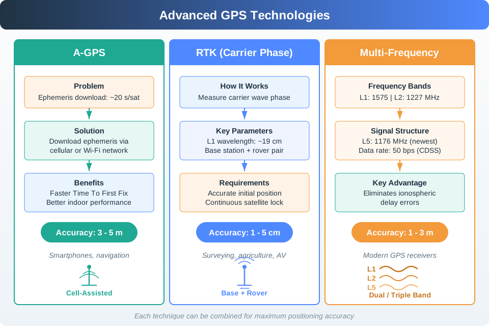
An accuracy upgrade matters only if it changes the connected-product decision. Start with the action, tolerance, confidence, update interval, cost, and recovery path, then decide whether DGPS, SBAS, RTK, PPP, or a simpler fix actually improves the user outcome.

Phoebe’s Field Notes: Why Errors Add in Quadrature, and Geometry Multiplies Them

Phoebe’s Why

This chapter’s UERE table adds six error sources by squaring, summing, and taking a square root instead of just adding them up – and that is not a rounding convenience, it is what independent random errors actually do. Each error source is roughly as likely to overshoot as undershoot, so when several add together, their bigger and smaller swings partly cancel; only the variances (not the errors themselves) are guaranteed to add. GDOP is a second, separate multiplier on top of that: it has nothing to do with the clocks or the ionosphere, and everything to do with where the four-plus satellites happen to be sitting in the sky when the receiver solves for position.

The Derivation

For independent random errors, variance adds, which is why root-sum-square, not linear addition, combines them:

\[\mathrm{Var}(\varepsilon_1+\varepsilon_2+\cdots)=\sigma_1^2+\sigma_2^2+\cdots \ \Rightarrow\ \mathrm{UERE}=\sqrt{\sigma_1^2+\sigma_2^2+\cdots+\sigma_6^2}\]

GDOP amplifies that per-satellite range error into position error through the satellite geometry matrix \(G\) (rows = unit line-of-sight vectors from receiver to each satellite):

\[\sigma_{position} = \mathrm{GDOP}\times\mathrm{UERE}, \qquad \mathrm{GDOP}=\sqrt{\mathrm{trace}\!\left[(G^{T}G)^{-1}\right]}\]

A minimal 2-D, 2-satellite toy version of that matrix shows why clustered satellites amplify error: for two line-of-sight directions separated by angle \(\varphi\), solving the same linear system gives a closed-form toy-DOP of

\[\mathrm{toy\text{-}DOP}(\varphi)=\frac{\sqrt2}{\sin\varphi}\]

smallest at \(\varphi=90°\) and diverging as the satellites line up (\(\varphi\to0°\) or \(180°\)).

Worked Numbers: This Chapter’s Own UERE and GDOP Numbers

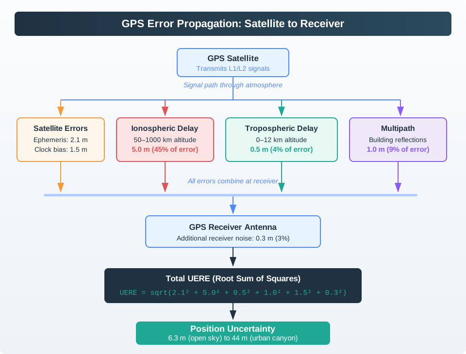
• Chapter’s six-source RSS: \(\sqrt{1.5^2+2.5^2+5.0^2+0.5^2+1.0^2+0.3^2}=\sqrt{34.8}=5.90\) m \(\approx6\) m, matching the chapter’s rounded UERE. Linear addition would give \(10.8\) m – \(1.83\times\) too pessimistic, which is exactly this chapter’s own “don’t simply add them up” point, now with the arithmetic behind it.
• Ionosphere’s share of the variance: \(5.0^2/34.8=71.8\%\approx72\%\), matching this chapter’s stated share.
• Position error is UERE times GDOP, not UERE plus GDOP: \(6\times1.5=9.00\) m (good geometry), \(6\times4.0=24.0\) m (this chapter’s own quiz), \(6\times6.5=39.0\) m (urban canyon) – this chapter’s own numbers all fall directly out of that one multiplication.
• Toy-DOP check: at \(\varphi=90°\) (satellites at right angles), \(\mathrm{toy\text{-}DOP}=\sqrt2/\sin90°=1.41\) – close to this chapter’s “good geometry” GDOP of 1.5. At \(\varphi=10°\) (nearly overhead-only satellites, this chapter’s own urban-canyon description), \(\mathrm{toy\text{-}DOP}=\sqrt2/\sin10°=8.14\) – in the same range as this chapter’s own 6.5-8.0 urban-canyon GDOP values, even though this toy model uses only two satellites in a flat plane. A real receiver runs the same amplification in three dimensions with more satellites; the toy model just makes visible why a clustered sky is the problem, not merely that it is.

35.2 Summary

GPS accuracy is controlled by error sources, satellite geometry, correction methods, receiver behavior, and the deployment environment. Accuracy design should match application risk and cost, from basic asset tracking to centimeter-level RTK control.

In 60 Seconds

Standard GPS achieves 5-10 meter accuracy under open sky, dominated by ionospheric delay (about 72% of the error variance, UERE²). Enhancement technologies dramatically improve this: DGPS removes common-mode errors to reach 0.5-1m, while RTK GPS uses carrier phase measurements for 1-2cm precision. The key design principle is matching accuracy to application – RTK for autonomous tractors planting 50cm rows, but basic GPS suffices for shipping container tracking.

35.3 Learning Objectives

By the end of this chapter, you will be able to:

• Analyze GPS Error Budget: Explain the contribution of each error source to total positioning uncertainty
• Calculate UERE: Apply root-sum-square to combine independent error sources into a single accuracy metric
• Compare Enhancement Technologies: Evaluate DGPS, SBAS, RTK, and PPP against specific accuracy requirements
• Design for Accuracy Requirements: Justify the selection of appropriate positioning technology for specific IoT applications

GPS Accuracy Basics

Standard GPS gives you 5-10 meter accuracy under open sky, but many IoT applications need much better. An autonomous tractor planting rows 50 cm apart needs centimeter precision, while a shipping container tracker is fine with 10 meters. This chapter breaks down where GPS errors come from (ionospheric delay is the biggest at about 72% of the error variance, UERE²) and how enhancement technologies fix them: DGPS gets you to 0.5-1 meter, while RTK GPS achieves 1-2 centimeter accuracy using carrier phase measurements. The key design principle is matching accuracy to your application – paying for RTK when basic GPS would suffice wastes power and money.

Key Concepts

• GPS: Global Positioning System providing 3-10 metre outdoor accuracy using triangulation from 4+ satellites, consuming 20-100 mA active current.
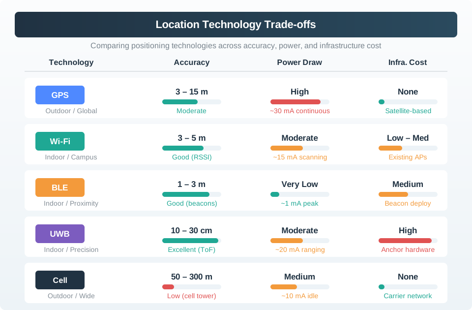
• Indoor Positioning: Techniques (BLE beacons, UWB, Wi-Fi RSSI, IMU dead-reckoning) achieving 0.1-5 metre accuracy where GPS signals are unavailable.
• Geofencing: Virtual geographic boundary triggering automated actions when a tracked asset enters or exits the defined area.
• Dead Reckoning: Position estimation using last known location plus measured movement (speed, heading) when GPS signal is lost.
• RSSI-Based Positioning: Location estimation from signal strength of known beacon nodes, achieving 2-5 metre accuracy in calibrated environments.
• Ultra-Wideband (UWB): Radio technology providing 10-30 cm indoor positioning accuracy using time-of-flight measurements between anchor nodes.
• Location Privacy: User right to control who can access their location history and how granular that location data is stored.

35.4 Prerequisites

• GPS and Outdoor Positioning: Understanding of GPS fundamentals and error sources

Chapter Roadmap

This chapter is long because location accuracy is both a measurement problem and a product promise.

1. First you decide what the user is allowed to trust from a location fix.
2. Then you break the fix into receiver state, geometry, correction data, and environment symptoms.
3. Next you calculate UERE and GDOP so the accuracy number is explainable.
4. After that you compare standard GPS, SBAS, DGPS, RTK, PPP, and indoor fallbacks against real IoT jobs.
5. Finally you check the cost, power, safety, quiz, and lab consequences of choosing the wrong tier.

Checkpoint callouts recap the main design decisions. Deep technical panels and calculators are useful references, but you can return to them after the first read.

35.5 Accuracy as Product Promise

First, treat accuracy as a contract between the system and the person acting on its output.

Location accuracy affects what a user is allowed to trust. A tracker that says a shipment is “at the depot” can tolerate a different error band from a campus robot that decides whether it is on a sidewalk, a farm machine that follows a crop row, or an emergency alert that chooses which building entrance to show responders.

Design the user experience around the useful accuracy interval, not the best number in a datasheet. The same GNSS receiver may report a good open-sky fix, a weak urban-canyon fix, a stale assisted-GPS estimate, or no fix indoors. The interface should make that state visible with bounded language such as “near loading bay 3,” “last seen 4 minutes ago,” or “centimeter guidance unavailable; manual steering required.”

Figure 35.1: Accuracy decisions trade precision against power, infrastructure, environment, and consequence; the best receiver is the one whose error state supports the product action.

• Fit for purpose: match the displayed precision to the task, cost, power budget, and risk of being wrong.
• State clarity: distinguish live fix, degraded fix, estimated position, and stale position before users act on it.
• Fallback: switch to Wi-Fi, BLE, UWB, IMU dead reckoning, computer vision, manual confirmation, or a safe stop when GNSS no longer supports the task.

The product promise should name the decision boundary. “Open the gate” might require enough confidence to know the vehicle is at the entrance and moving slowly. “Show a child at school” might need a zone and a recent timestamp, not an exact coordinate. “Guide a tractor row” might require a fixed RTK state and an alarm when correction data is stale. The same latitude and longitude can be acceptable for one feature and unsafe for another.

Accuracy also changes over time. Satellite geometry shifts, antennas are shadowed by a trailer or building, leaves and wet glass create multipath, a correction stream ages, and an indoor handoff may depend on Wi-Fi, BLE, UWB, barometer, or IMU data. A good interface does not show extra decimal places just because the API returns them. It shows uncertainty circles, zone labels, stale markers, disabled buttons, confidence bands, or manual confirmation when the error estimate crosses a product threshold.

For IoT designers, the important question is usually not “what is the most accurate technology?” It is “what is the cheapest, lowest-power, maintainable signal that keeps the feature honest?” Shipping containers, delivery fleets, farm guidance, drones, indoor assets, personal safety wearables, and campus robots can all need different combinations of GNSS, SBAS, DGPS, RTK, PPP, Wi-Fi positioning, BLE proximity, UWB ranging, vision, lidar, and human confirmation.

35.6 Accuracy UI Rules

Start with the action that location enables. For a shipping container, the question may be “which yard or gate?” For a delivery driver, it may be “which side of the street?” For precision agriculture, it may be “is the tractor centered within a few centimeters?” Each action needs a stated tolerance, update interval, confidence level, fallback, and user message.

Useful implementation signals include HDOP or GDOP, estimated horizontal and vertical accuracy, fix type, satellite count, correction age, carrier-phase fix status, time since last fix, speed, heading, battery state, antenna fault, and whether the receiver is using standalone GNSS, SBAS such as WAAS or EGNOS, DGPS, RTK, PPP, or sensor fusion. Store those signals with the location event so support staff can see why the product showed a coarse zone instead of an exact point.

1. Write a tolerance table: connect each feature to a maximum horizontal error, vertical error if relevant, update cadence, and allowed fallback.
2. Choose honest display language: show zones, uncertainty circles, “last known” timestamps, or disabled controls when the fix does not meet the tolerance.
3. Test hard places: include open sky, tree cover, warehouse entrances, street canyons, tunnels, high-rise approaches, and indoor handoff points.

Translate the tolerance table into UI states and automation guards. A dashboard might show a green “RTK fixed” badge only when correction age, satellite count, and covariance are inside bounds. A mobile app might label a delivery as “near the entrance” instead of pinning it to a door when the reported horizontal accuracy is wider than the building frontage. A robot controller might slow down, request vision confirmation, or stop when the uncertainty radius overlaps a curb, crop row, loading dock edge, or restricted zone.

Field validation should use representative routes, not a lab bench alone. Walk or drive the system through open fields, metal warehouses, tree cover, alleyways, tunnels, parking structures, high-rise entrances, and transition zones between outdoor GNSS and indoor positioning. Record the displayed state, raw receiver state, correction source, power draw, network availability, and user action taken. Those traces become regression tests for later firmware, antenna, map, or dashboard changes.

Cost review belongs in the same design pass. RTK can be justified when centimeter error prevents crop damage, grading mistakes, or unsafe vehicle movement, but it may be wasteful for asset tracking or large geofence alerts. Conversely, a cheap receiver is not cheap if it causes false arrivals, missed stops, manual dispatch calls, damaged products, or unsafe robot behavior. The design record should state why the chosen accuracy tier is enough and what the system does when it is not enough.

Checkpoint: Product Accuracy Contract

You now know:

• The right accuracy is the one that supports the product action, not the smallest number in a datasheet.
• A location event should carry fix state, confidence, stale time, correction status, and fallback language.
• Field tests must include the hard places where users actually depend on the result.

35.7 Corrections Need Visible Errors

Now connect that product contract to the signals coming out of the receiver and correction service.

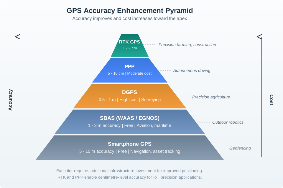
GNSS accuracy is built from measurement quality, satellite geometry, correction data, and receiver state. L1/L2/L5 measurements, GPS/Galileo/GLONASS/BeiDou satellite availability, C/N0 signal quality, ephemeris age, ionospheric and tropospheric models, multipath rejection, antenna placement, and receiver clock behavior all affect the reported fix. SBAS broadcasts wide-area corrections. DGPS uses a nearby reference station. RTK uses carrier-phase measurements and needs continuous lock. PPP relies on precise orbit and clock products and usually has convergence time.

The system boundary matters as much as the math. RTK correction streams may arrive over NTRIP using RTCM 3 messages, local radios, or a vendor cloud service. If the correction age grows, the rover loses fixed status, the antenna is shadowed, or the receiver falls back from RTK fixed to float or standalone GNSS, the product must stop presenting centimeter-level confidence. Logs should preserve fix type, covariance or accuracy estimate, correction source, correction age, geofence decision, command id, map-matching result, and the message shown to the user.

• Correction scope: DGPS and SBAS reduce shared satellite, clock, and atmospheric errors; they do not remove local multipath from glass, metal, trees, or bad antenna placement.
• Safety boundary: when error exceeds the clearance needed for steering, docking, routing, or emergency response, slow down, ask for confirmation, or switch control mode.
• Privacy boundary: collect only the accuracy needed for the feature; a zone event can be enough when a continuous coordinate trail would expose unnecessary movement history.

Mathematically, the receiver is estimating position from noisy range observations. UERE captures range error sources, while DOP describes how satellite geometry amplifies those errors into position uncertainty. A low-noise receiver with poor geometry can still produce a poor position. A good correction stream cannot remove a reflection from a nearby wall if the antenna receives a delayed signal path. That is why reliable products track both source quality and environment symptoms.

Sensor fusion adds another layer of contracts. An extended Kalman filter or similar estimator can combine GNSS, wheel odometry, IMU acceleration, magnetometer heading, barometer altitude, camera lane detection, lidar obstacles, Wi-Fi fingerprints, BLE proximity, and UWB ranges. The fused output should expose covariance, source contributors, last update time, and fault flags so downstream automation can decide whether the estimate is suitable for display, routing, steering, billing, or only historical logging.

Persistence should keep enough evidence to debug bad decisions without storing unnecessary movement history. A compact event can include fix_type, horizontal_accuracy, vertical_accuracy, hdop, satellite_count, correction_age, correction_source, map_version, fusion_mode, confidence, stale_after, and the user-visible label. For privacy-sensitive features, store a zone or decision result unless raw coordinates are required for a short-lived operational reason.

Checkpoint: Error Evidence

You now know:

• SBAS, DGPS, RTK, and PPP improve different parts of the error stack.
• Local multipath, blocked antennas, correction age, and fix type still have to be surfaced to the product.
• Logs should preserve enough evidence to explain why the interface showed a zone, warning, disabled control, or precise point.

35.8 GPS Error Budget Basics

With the contract and evidence fields in place, the next question is how to calculate the error number itself.

Understanding where GPS accuracy comes from—and where it breaks down—is critical for designing reliable IoT location services. A GPS error budget quantifies each error source’s contribution to total positioning uncertainty.

35.8.1 Error Budget Breakdown

The table below shows the six main error sources, their typical magnitude, how variable they are, and how we can mitigate them:

Error Source	Typical Error	Notes
Satellite clock	1.5 m	Atomic clock drift compensated by ground uploads every 15 minutes
Ephemeris data	2.5 m	Orbital prediction errors; frequent updates every 2 hours minimize drift
Ionospheric delay	5.0 m	Varies with solar activity; equatorial regions 2-3× worse than poles
Tropospheric delay	0.5 m	Weather dependent; humidity and temperature affect signal propagation
Multipath	1.0 m	Urban canyons worst case; signals bounce off buildings creating echoes
Receiver noise	0.3 m	Hardware quality dependent; better RF front-ends reduce noise floor
Total (UERE)	~6 m	Root sum square of all independent error sources
With DGPS	<1 m	Differential correction removes common-mode errors (ionosphere, clock)
With RTK	<2 cm	Real-time kinematic uses carrier phase for centimeter-level precision

Understanding Error Accumulation

GPS errors don’t simply add up—they combine using root sum square (RSS) because they’re independent random variables:

\[ \text{UERE} = \sqrt{1.5^2 + 2.5^2 + 5.0^2 + 0.5^2 + 1.0^2 + 0.3^2} \approx 6 \text{ meters} \]

Why RSS and not simple addition? If errors added linearly, total would be 10.8 meters. But some errors cancel each other out randomly, resulting in the more realistic 6-meter UERE.

Putting Numbers to It

Let’s calculate the actual error budget for a GPS receiver in three different environments to see how context affects accuracy.

Scenario 1: Rural open sky (best case)

Given error sources: - Satellite clock: \(\sigma_{\text{clock}} = 1.5\) m - Ephemeris: \(\sigma_{\text{eph}} = 2.5\) m - Ionosphere: \(\sigma_{\text{iono}} = 3.0\) m (low solar activity, mid-latitude) - Troposphere: \(\sigma_{\text{tropo}} = 0.5\) m - Multipath: \(\sigma_{\text{mp}} = 0.3\) m (no reflective surfaces) - Receiver noise: \(\sigma_{\text{rx}} = 0.3\) m

\[ \text{UERE} = \sqrt{1.5^2 + 2.5^2 + 3.0^2 + 0.5^2 + 0.3^2 + 0.3^2} = \sqrt{17.93} \approx 4.2 \text{ m} \]

With excellent satellite geometry (GDOP = 1.5):

\[ \text{Position error} = 4.2 \times 1.5 \approx \mathbf{6.3 \text{ meters}} \]

Scenario 2: Urban canyon (worst case)

Same base errors, but: - Ionosphere: \(\sigma_{\text{iono}} = 5.0\) m (standard) - Multipath: \(\sigma_{\text{mp}} = 3.5\) m (signals bounce off glass buildings)

\[ \text{UERE} = \sqrt{1.5^2 + 2.5^2 + 5.0^2 + 0.5^2 + 3.5^2 + 0.3^2} = \sqrt{46.09} \approx 6.8 \text{ m} \]

Poor satellite geometry (only 4 satellites visible overhead, GDOP = 6.5):

\[ \text{Position error} = 6.8 \times 6.5 \approx \mathbf{44 \text{ meters!}} \]

Scenario 3: Equatorial region, solar storm

• Ionosphere: \(\sigma_{\text{iono}} = 12.0\) m (extreme solar activity)

\[ \text{UERE} = \sqrt{1.5^2 + 2.5^2 + 12.0^2 + 0.5^2 + 1.0^2 + 0.3^2} = \sqrt{153.84} \approx 12.4 \text{ m} \]

With GDOP = 2.0:

\[ \text{Position error} = 12.4 \times 2.0 \approx \mathbf{25 \text{ meters}} \]

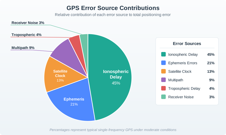
Key insight: The same GPS receiver ranges from 6.3m accuracy (rural) to 44m (urban canyon) purely due to environment. Ionospheric delay dominates the error variance – about 72% of UERE² under typical mid-latitude conditions, rising to roughly 94% during a solar storm (each source’s share is its variance divided by UERE², so the shares sum to 100% of UERE²).

Figure 35.2: Pie chart showing relative contribution of GPS error sources to total positioning error.

Figure 35.3: Flowchart showing how GPS errors propagate from satellite to receiver.

Ionospheric GPS Error Share

The ionosphere (50-1000 km altitude) is a layer of charged particles created by solar radiation. GPS signals travel through it, and the charged particles slow down the radio waves, making distances appear longer.

Why it’s variable:

• Solar activity: During solar storms, ionospheric delay can spike to 10-15 meters (vs. 5m typical)
• Time of day: Peak ionization occurs at noon (sun overhead), minimum at night
• Geographic location: Equatorial regions have 2-3× higher ionospheric activity than poles

Mitigation:

• Dual-frequency receivers: Military (L1 + L2) and modern smartphones (L1 + L5) measure two frequencies and calculate ionospheric delay directly
• SBAS augmentation: WAAS (North America), EGNOS (Europe) broadcast ionospheric models
• Single-frequency compromise: Civilian L1-only receivers use Klobuchar model (removes ~50% of error)

35.8.2 Calculating Total GPS Uncertainty (UERE)

UERE (User Equivalent Range Error) is the root-sum-square (RSS) of all error sources, assuming they’re independent and random:

\[ \text{UERE} = \sqrt{\sigma_{\text{clock}}^2 + \sigma_{\text{eph}}^2 + \sigma_{\text{iono}}^2 + \sigma_{\text{tropo}}^2 + \sigma_{\text{multipath}}^2 + \sigma_{\text{noise}}^2} \]

Plugging in typical values:

\[ \text{UERE} = \sqrt{1.5^2 + 2.5^2 + 5.0^2 + 0.5^2 + 1.0^2 + 0.3^2} = \sqrt{2.25 + 6.25 + 25.0 + 0.25 + 1.0 + 0.09} \]

\[ \text{UERE} = \sqrt{34.84} \approx \mathbf{6 \text{ meters}} \]

Interactive UERE Calculator

Adjust the error sources below to see how they affect total GPS uncertainty:

viewof clockError = Inputs.range([0, 5], {value: 1.5, step: 0.1, label: "Satellite Clock Error (m)"})
viewof ephemerisError = Inputs.range([0, 5], {value: 2.5, step: 0.1, label: "Ephemeris Error (m)"})
viewof ionosphericError = Inputs.range([0, 15], {value: 5.0, step: 0.5, label: "Ionospheric Delay (m)"})
viewof troposphericError = Inputs.range([0, 2], {value: 0.5, step: 0.1, label: "Tropospheric Delay (m)"})
viewof multipathError = Inputs.range([0, 5], {value: 1.0, step: 0.1, label: "Multipath Error (m)"})
viewof receiverNoise = Inputs.range([0, 2], {value: 0.3, step: 0.1, label: "Receiver Noise (m)"})

uere = Math.sqrt(
  Math.pow(clockError, 2) +
  Math.pow(ephemerisError, 2) +
  Math.pow(ionosphericError, 2) +
  Math.pow(troposphericError, 2) +
  Math.pow(multipathError, 2) +
  Math.pow(receiverNoise, 2)
)

viewof gdop = Inputs.range([1, 10], {value: 2.0, step: 0.1, label: "GDOP (Geometric Dilution of Precision)"})

positionError = uere * gdop

html`<div style="background: #2C3E50; color: white; padding: 20px; border-radius: 8px; margin-top: 15px; font-family: Arial, sans-serif;">
  <div style="font-size: 24px; font-weight: bold; margin-bottom: 10px;">
    UERE = ${uere.toFixed(2)} meters
  </div>
  <div style="font-size: 18px; color: #16A085; margin-bottom: 15px;">
    Position Error = UERE × GDOP = ${uere.toFixed(2)} × ${gdop.toFixed(1)} = ${positionError.toFixed(1)} meters
  </div>
  <div style="font-size: 14px; opacity: 0.9;">
    <strong>Error Breakdown:</strong><br/>
    Ionospheric: ${((Math.pow(ionosphericError, 2) / Math.pow(uere, 2)) * 100).toFixed(1)}% |
    Ephemeris: ${((Math.pow(ephemerisError, 2) / Math.pow(uere, 2)) * 100).toFixed(1)}% |
    Clock: ${((Math.pow(clockError, 2) / Math.pow(uere, 2)) * 100).toFixed(1)}% |
    Multipath: ${((Math.pow(multipathError, 2) / Math.pow(uere, 2)) * 100).toFixed(1)}% |
    Tropospheric: ${((Math.pow(troposphericError, 2) / Math.pow(uere, 2)) * 100).toFixed(1)}% |
    Receiver: ${((Math.pow(receiverNoise, 2) / Math.pow(uere, 2)) * 100).toFixed(1)}%
  </div>
</div>`

Try these scenarios:

• Open sky, good conditions: Set ionospheric = 3m, multipath = 0.3m, GDOP = 1.5 → ~6.3m accuracy
• Urban canyon: Set ionospheric = 5m, multipath = 3.5m, GDOP = 6.5 → ~44m accuracy
• Solar storm: Set ionospheric = 12m, GDOP = 2.0 → ~25m accuracy

UERE, GDOP, and Position Error

UERE (6 meters) is the range error per satellite. Your actual position error depends on satellite geometry (GDOP):

\[ \text{Position Error} = \text{UERE} \times \text{GDOP} \]

• Good geometry (satellites spread across sky): GDOP ≈ 1.5 → Position error ≈ 9 meters
• Poor geometry (satellites clustered): GDOP ≈ 3.0 → Position error ≈ 18 meters
• Urban canyon (only overhead satellites visible): GDOP ≈ 8.0 → Position error ≈ 48 meters!

This is why GPS accuracy in downtown Manhattan (tall buildings) can degrade to 50+ meters, while open-sky rural areas achieve 3-5 meters.

Checkpoint: UERE and GDOP

You now know:

• UERE combines independent range errors with root-sum-square arithmetic.
• GDOP multiplies that range error, so poor geometry can turn the same receiver into a much worse position estimate.
• Environment changes matter: open sky, urban canyon, and solar storm scenarios produce very different expected errors.

35.8.3 Accuracy from Phones to Agriculture

Once the math is visible, the design choice becomes a tiering decision.

Different IoT applications require different levels of positioning accuracy. Here’s how various technologies stack up:

Technology	Typical Accuracy	Setup Requirements	Cost	Common IoT Use Cases
Smartphone GPS	5-10 m	None (standalone)	Free	Navigation, asset tracking, geofencing
SBAS (WAAS/EGNOS)	1-3 m	None (broadcast)	Free	Aviation, maritime navigation, outdoor robotics
DGPS	0.5-1 m	Base station + radio link	\[$ (infrastructure) | **Surveying**, precision agriculture, autonomous vehicles | | **RTK GPS** | 1-2 cm | Base station + continuous radio | \]\[ (equipment + subscription) | **Precision farming** (tractors), construction, drone surveying | | **PPP (Precise Point Positioning)** | 5-10 cm | Internet connection | \] (subscription)	Surveying, geophysical monitoring, autonomous driving

Figure 35.4: Pyramid diagram showing GPS accuracy levels and applications.

Choose GPS Accuracy for IoT

Match accuracy to application requirements—don’t over-engineer!

Application	Required Accuracy	Recommended Technology	Why
Asset tracking (shipping containers)	10 m	Standard GPS	Just need to know “which warehouse” or “which city”—5-10m is overkill
Fleet management (delivery trucks)	3 m	SBAS (WAAS)	Need to distinguish which side of street vehicle is on
Precision agriculture (autonomous tractor)	2 cm	RTK GPS	Row spacing is 30-76 cm—need sub-decimeter accuracy to avoid crop damage
Drone surveying	5 cm	PPP or RTK	Generating topographic maps requires centimeter-level vertical accuracy
Indoor warehouse	N/A	Wi-Fi/UWB	GPS doesn’t work indoors—need alternative positioning system

Indoor Positioning Reality Check:

• GPS signals are −130 dBm (extremely weak) outdoors
• Building materials attenuate signals by 20-40 dB
• Result: No GPS fix indoors in most buildings (concrete, steel)
• Solution: Use Wi-Fi fingerprinting (5-15m), BLE beacons (1-3m), or UWB (10-30cm) instead

Common GPS Accuracy Misconceptions

Myth 1: “GPS is always accurate to within 5 meters” - Reality: 5-10m is open-sky accuracy. Urban canyons (tall buildings) can degrade accuracy to 50+ meters due to multipath and poor GDOP.

Myth 2: “More satellites = better accuracy” - Reality: Satellite geometry matters more than count. 4 widely-spaced satellites (GDOP = 1.5) beat 8 clustered satellites (GDOP = 4.0).

Myth 3: “Differential GPS eliminates all errors” - Reality: DGPS only corrects common-mode errors (ionosphere, satellite clock) that affect base and mobile identically. It doesn’t fix multipath (location-specific) or receiver noise.

Myth 4: “RTK gives 2cm accuracy everywhere” - Reality: RTK requires continuous phase lock to satellites. Driving under bridges, trees, or tunnels breaks lock and accuracy degrades to standard GPS (5-10m) until lock is re-established.

Checkpoint: Accuracy Tiers

You now know:

• Standard GPS, SBAS, DGPS, RTK, PPP, Wi-Fi, BLE, and UWB solve different accuracy and environment problems.
• Over-engineering wastes power, infrastructure, and subscription budget.
• Under-engineering creates false arrivals, unsafe automation, and manual support work.

35.9 Differential GPS (DGPS)

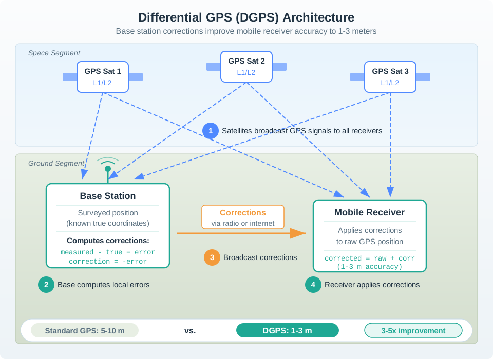
The first enhancement tier is differential correction: use a known reference to cancel shared outdoor GNSS errors.

Figure 35.5: Diagram showing DGPS system with base station broadcasting corrections to mobile receivers.

DGPS Principle:

1. Base Stations at Known Locations:
   • Precisely surveyed reference positions
   • Distributed around the world
2. Base Stations Calculate Local Errors:
   • Position themselves using GPS
   • Compare to known true position
   • Model local GNSS errors
3. Transmit Corrections:
   • Broadcast corrections out-of-band (radio, internet)
   • Local receivers apply same corrections
   • Accuracy: 1-3 meters (vs 5-10m for standard GPS)

Historical Note:

• Came about due to US “Selective Availability” (SA)
• SA: Intentional GPS errors for security (civilians got degraded service)
• SA turned off in May 2000
• DGPS still valuable for removing natural errors

35.10 Advanced GPS Techniques

Figure 35.6: Diagram showing three advanced GPS technologies: A-GPS, RTK, and multi-frequency signals.

1. Assisted-GPS (A-GPS):

• Problem: Downloading ephemeris (satellite orbital data) takes ~20s per satellite
• Solution: Get ephemeris via cellular or Wi-Fi data connection
• Benefit: Faster Time To First Fix (TTFF), works indoors better

2. Carrier Phase Positioning (RTK):

• GPS signal wavelength: ~19 cm (L1 band at 1575 MHz)
• Measure phase of carrier wave (not just code)
• Accuracy: Centimeter-level (2-5 cm)
• Requirements:
  • Very accurate initial location
  • Observe satellites for extended period
  • Maintain continuous lock (no “cycle slips”)
• Applications: Surveying, precision agriculture, autonomous vehicles

3. Signal Structure:

• Multiple frequency bands: L1 (1575 MHz), L2 (1227 MHz), L5 (1176 MHz)
• Data rate: Only 50 bits per second (very slow!)
• Uses spread-spectrum (CDSS) for signal strength and interference resistance

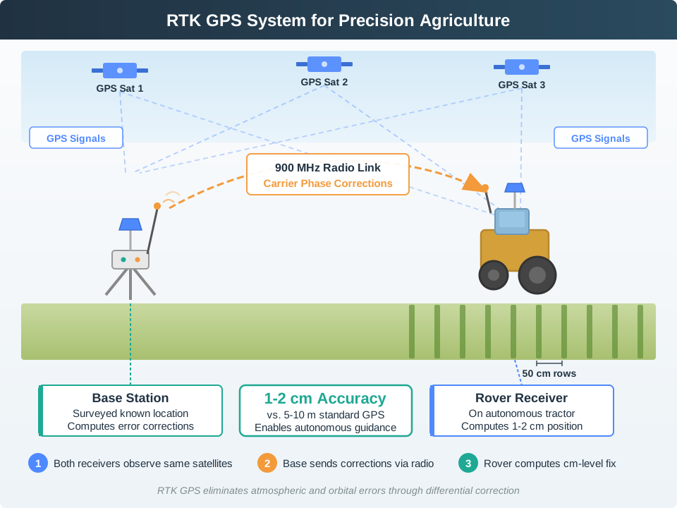
35.11 RTK GPS in Precision Agriculture

RTK is the chapter’s clearest example of accuracy as a business and safety requirement rather than a luxury specification.

Understanding when augmentation (DGPS, RTK) is needed is critical for IoT system design. Let’s examine a real-world precision agriculture case where centimeter-level accuracy is mandatory.

Autonomous Tractor Guidance

Problem: Modern farms use autonomous tractors for planting and harvesting. Crop rows are spaced 30-76 cm (12-30 inches) apart. Standard GPS (5-10 meter accuracy) would cause the tractor to:

• Destroy crops: Driving over planted rows instead of between them
• Miss coverage: Leaving gaps in planting or harvesting
• Overlap excessively: Wasting seeds, fertilizer, and fuel

Why Standard GPS Fails:

Technology	Accuracy	Can Navigate 50cm Rows?	Result
Smartphone GPS	5-10 m	No	10× too imprecise—tractor wanders across 20 rows
DGPS	0.5-1 m	No	Still 2× too large—damages crops on both sides
RTK GPS	1-2 cm	Yes	Pass-to-pass accuracy maintains lane position

Solution: RTK GPS provides sub-2cm accuracy enabling:

• Straight-line guidance: Maintain row centerline within ±2 cm over 1 km runs
• Repeat passes: Return to exact same tracks on subsequent operations (planting → spraying → harvesting)
• Nighttime operation: Autonomous 24/7 operation without visual references
• Reduced overlap: Typical 5-10% overlap reduced to 1-2% (saves $25,000-$50,000/year on 1000-acre farm in fuel, seeds, chemicals)

Figure 35.7: Diagram showing RTK GPS setup for autonomous tractor with base station and rover receiver.

RTK vs DGPS vs Standard GPS

Decision Framework for IoT Location Systems:

Application Requirement	Recommended Technology	Typical Cost	Justification
Row-crop farming (30-76 cm rows)	RTK GPS	$15,000-$25,000	1-2 cm accuracy required; ROI in 1-2 years from reduced overlap
Broadcast fertilizing (no rows)	DGPS	$2,000-$5,000	0.5-1 m sufficient to avoid coverage gaps and excessive overlap
Livestock tracking (which pasture?)	Standard GPS	$50-$200	5-10 m accuracy adequate; just need geofence boundaries
Construction grading (±2 cm elevation)	RTK GPS + tilt sensors	$20,000-$40,000	Vertical accuracy critical for drainage and leveling
Drone surveying (topographic maps)	RTK GPS or PPP	$5,000-$15,000	Centimeter-level required for accurate 3D models
Fleet delivery tracking	Smartphone GPS	Free (built-in)	Know which city block vehicle is on; 5-10m sufficient

Key Insight: Match accuracy to application—don’t over-engineer! RTK GPS costs 10-50× more than standard GPS. Only use it when centimeter-level precision delivers measurable ROI.

RTK GPS Limitations in IoT Deployments

Common Pitfalls When Designing RTK Systems:

1. Requires Continuous Radio Link (Base ↔︎ Rover):
   • Problem: Hills, trees, buildings block 900 MHz/2.4 GHz radio
   • Range limit: Typically 10 km line-of-sight, much less in rugged terrain
   • Solution: Deploy multiple base stations or use NTRIP (internet-based corrections)
2. Loses Accuracy if Satellite Lock Breaks:
   • Problem: Driving under trees, bridges, or in narrow canyons causes “cycle slips”
   • Recovery time: 30 seconds to several minutes to re-establish centimeter fix
   • Fallback: System degrades to DGPS (1m) or standard GPS (5-10m) during outages
3. Expensive and Power-Hungry:
   • Base station: 5-15 watts continuous power (requires AC or large solar panel)
   • Rover receiver: 2-5 watts (vs. 0.5W for standard GPS)
   • Total system cost: $15,000-$25,000 (base + rover + radio + installation)
4. Requires Expertise to Set Up:
   • Base station must be surveyed to ±1 cm accuracy (professional surveyor)
   • Radio frequency coordination (avoid interference with other farm equipment)
   • Antenna placement (clear sky view, stable mounting, lightning protection)

When RTK is NOT Worth It:

• Wrong: Use RTK to track shipping containers (5-10m GPS sufficient to know “which warehouse”)
• Wrong: Track hospital wheelchairs indoors (GPS doesn’t work indoors; use BLE beacons instead)
• Right: Autonomous tractors planting 50cm rows ($40,000/year savings justifies $20,000 equipment)

Checkpoint: Enhancement Selection

You now know:

• DGPS improves nearby outdoor receivers by correcting shared errors.
• RTK needs continuous carrier-phase lock, correction delivery, and clear enough sky to keep centimeter confidence.
• The right selection record states the accuracy tier, cost, power, fallback mode, and failure message.

35.12 Knowledge Check

Quiz: GPS Accuracy and Enhancement

GPS Tech Cost Decisions

Illustrative Cost Comparison:

Two modeled IoT deployments illustrate the importance of matching accuracy to application. Treat these numbers as planning assumptions for comparing orders of magnitude, not as claims from a named deployment:

Scenario	Requirement	Technology	Cost	ROI
Last-Mile Delivery Fleet (200 trucks)	10m accuracy to know which city block	Standard smartphone GPS	$19,200/year (cellular data only)	$45,000/year fuel savings from optimized routing
Autonomous Tractor Farm (4 tractors, 2,000 acres)	2cm accuracy for 50cm row spacing	RTK GPS system	$40,800 upfront + $2,400/year	$117,000/year savings (8% overlap reduction + 24/7 operation), 4.3-month payback

Key insight: In this model, the delivery fleet would waste money on unnecessary RTK precision. The tractor deployment would carry large operational risk if standard GPS were used for row guidance.

GPS Technology Selection by Application:

Application	Accuracy Needed	Recommended Technology	Typical Cost/Unit	Key Constraint
Shipping container tracking	10-50 m (city-level)	Standard GPS	$50-150	Battery life (years), not accuracy
Delivery fleet management	5-10 m (street-level)	Standard GPS + SBAS	$0-200	Free GPS in phones sufficient
Autonomous lawnmower	10-20 cm (avoid flower beds)	RTK GPS or PPP	$1,500-4,000	Needs obstacle avoidance sensors too
Precision seeding tractor	1-2 cm (50cm row spacing)	RTK GPS with base station	$8,000-15,000	Must maintain continuous phase lock
Construction grading	2-5 cm (drainage requirements)	RTK GPS + tilt sensors	$15,000-30,000	Vertical accuracy critical
Drone surveying	5-10 cm (topographic mapping)	RTK or PPP	$3,000-8,000	Weight/power constraints
Personal fitness tracker	3-10 m (route tracking)	Standard GPS (smartphone)	Free	Battery life, not accuracy
Geofencing (entry/exit zones)	10-30 m (zone boundaries)	Standard GPS	Free	Zone design compensates for accuracy

Cost-benefit decision tree:

1. Is <5m accuracy ESSENTIAL for function?
   • No → Use standard GPS ($0-200/unit)
   • Yes → Continue to question 2
2. Is <10cm accuracy ESSENTIAL?
   • No → Use DGPS or SBAS ($0-500/unit for receiver)
   • Yes → Continue to question 3
3. Can you deploy a base station?
   • Yes → Use RTK GPS ($8,000-15,000/unit + $10,000 base shared across all units)
   • No → Use PPP ($2,000-5,000/unit + $50-200/month subscription)
4. Is real-time required?
   • Yes → Must use RTK or real-time PPP (requires radio or cell connection)
   • No → Can use post-processed PPP (acceptable for surveying, not for autonomous vehicles)

Power/cost tradeoff:

• Standard GPS: 0.5W continuous
• RTK GPS: 2-5W continuous (processing carrier phase)
• For battery-powered devices, accuracy comes at 4-10× power cost

Interactive RTK ROI Calculator

Calculate the return on investment for RTK GPS in precision agriculture:

viewof farmAcres = Inputs.range([100, 5000], {value: 2000, step: 100, label: "Farm Size (acres)"})
viewof numTractors = Inputs.range([1, 10], {value: 4, step: 1, label: "Number of Tractors"})
viewof overlapReduction = Inputs.range([0, 15], {value: 8, step: 1, label: "Overlap Reduction (%)"})
viewof fuelPrice = Inputs.range([2, 8], {value: 4, step: 0.25, label: "Diesel Price ($/gallon)"})

// RTK System Costs
baseStationCost = 8500
roverCost = 6200
radioCost = 2800
surveyCost = 1500
installCost = 3200
totalUpfront = baseStationCost + (roverCost * numTractors) + radioCost + surveyCost + installCost
annualMaintenance = 2400

// Annual Savings Calculations
fuelSavingsPerAcre = 2.5 // gallons per acre baseline
fuelSavings = farmAcres * fuelSavingsPerAcre * (overlapReduction / 100) * fuelPrice

seedSavingsPerAcre = 9 // dollars per acre
seedSavings = farmAcres * seedSavingsPerAcre * (overlapReduction / 100)

fertilizerSavingsPerAcre = 11 // dollars per acre
fertilizerSavings = farmAcres * fertilizerSavingsPerAcre * (overlapReduction / 100)

laborSavings = numTractors * 16250 // $65k/year per tractor reduced by 25%

totalAnnualSavings = fuelSavings + seedSavings + fertilizerSavings + laborSavings
netAnnualSavings = totalAnnualSavings - annualMaintenance
paybackMonths = (totalUpfront / netAnnualSavings) * 12

html`<div style="background: linear-gradient(135deg, #2C3E50 0%, #34495e 100%); color: white; padding: 25px; border-radius: 8px; margin-top: 15px; font-family: Arial, sans-serif;">
  <div style="display: grid; grid-template-columns: 1fr 1fr; gap: 20px; margin-bottom: 20px;">
    <div style="background: rgba(255,255,255,0.1); padding: 15px; border-radius: 6px;">
      <div style="font-size: 14px; opacity: 0.8; margin-bottom: 5px;">Total Upfront Cost</div>
      <div style="font-size: 28px; font-weight: bold; color: #E67E22;">$${totalUpfront.toLocaleString()}</div>
      <div style="font-size: 12px; opacity: 0.7; margin-top: 5px;">
        Base: $${baseStationCost.toLocaleString()} | Rovers: $${(roverCost * numTractors).toLocaleString()} | Other: $${(radioCost + surveyCost + installCost).toLocaleString()}
      </div>
    </div>
    <div style="background: rgba(255,255,255,0.1); padding: 15px; border-radius: 6px;">
      <div style="font-size: 14px; opacity: 0.8; margin-bottom: 5px;">Payback Period</div>
      <div style="font-size: 28px; font-weight: bold; color: #16A085;">${paybackMonths.toFixed(1)} months</div>
      <div style="font-size: 12px; opacity: 0.7; margin-top: 5px;">
        Annual Maintenance: $${annualMaintenance.toLocaleString()}/year
      </div>
    </div>
  </div>
  <div style="background: rgba(22, 160, 133, 0.2); padding: 15px; border-radius: 6px; border-left: 4px solid #16A085;">
    <div style="font-size: 16px; font-weight: bold; margin-bottom: 10px;">Annual Savings Breakdown:</div>
    <div style="display: grid; grid-template-columns: repeat(2, 1fr); gap: 10px; font-size: 14px;">
      <div>🚜 Fuel: $${fuelSavings.toLocaleString()}</div>
      <div>🌱 Seeds: $${seedSavings.toLocaleString()}</div>
      <div>🧪 Fertilizer: $${fertilizerSavings.toLocaleString()}</div>
      <div>👷 Labor: $${laborSavings.toLocaleString()}</div>
    </div>
    <div style="margin-top: 15px; padding-top: 15px; border-top: 1px solid rgba(255,255,255,0.2); font-size: 18px; font-weight: bold;">
      Total Annual Savings: $${totalAnnualSavings.toLocaleString()} (Net: $${netAnnualSavings.toLocaleString()})
    </div>
  </div>
  <div style="margin-top: 15px; font-size: 13px; opacity: 0.8; text-align: center;">
    ${paybackMonths < 6 ? "✅ Excellent ROI - RTK system pays for itself in under 6 months" :
      paybackMonths < 12 ? "✅ Good ROI - RTK system pays for itself within a year" :
      paybackMonths < 24 ? "⚠️ Moderate ROI - Consider farm size and labor costs" :
      "❌ Poor ROI - Standard GPS or DGPS may be more cost-effective"}
  </div>
</div>`

Insights: Under the calculator’s default assumptions, payback falls in the 4-8 month range because overlap reduction and labor assumptions dominate the result. Smaller farms, lower overlap reduction, or higher maintenance costs can push the payback period much longer.

GPS Limits in Safety Navigation

The mistake: Using standard 5-10m GPS accuracy for applications where centimeter precision prevents accidents or damage.

Illustrative scenario 1: Autonomous Vineyard Sprayer A vineyard purchased an autonomous sprayer with standard GPS (5-10m accuracy). Vine rows were spaced 2.5 meters apart.

Failure mode: GPS error could cause the sprayer to: - Drive over 12 rows of grapevines (15% of vineyard section) - Spray adjacent properties (chemical trespass lawsuit) - Get stuck in irrigation ditch (not detected, 8m off course)

Modeled impact: $85,000 in destroyed vines, $22,000 legal settlement, and $8,000 equipment recovery.

Root cause: Project manager didn’t understand GPS accuracy vs. row spacing. Assumed “GPS-guided” was sufficient without checking precision spec.

What RTK would have prevented: 2cm accuracy keeps sprayer centered in 2.5m rows with 1.23m clearance on each side. Even with 10cm error (degraded RTK), still 1.15m clearance—safe.

Illustrative scenario 2: Autonomous Delivery Robot A campus delivery robot used standard smartphone GPS (5-10m accuracy) to navigate sidewalks (1.5m wide).

Failure mode: GPS error could cause the robot to: - Drive onto grass (got stuck 8 times in first week) - Block wheelchair access ramps (ADA complaint) - Enter vehicle traffic lane (3m GPS error made it think it was on parallel sidewalk)

Modeled impact: Program suspended after 2 weeks, with $120,000 in development effort stranded.

The fix: Sensor fusion

• Standard GPS for coarse positioning (which campus area?)
• Computer vision for sidewalk edge detection (stay within 1.5m path)
• Lidar for obstacle avoidance (don’t hit people)
• Lesson: Safety-critical navigation requires GPS PLUS other sensors, never GPS alone

Warning signs your project needs better GPS:

1. Clearance < 10× GPS accuracy: Rows 50cm apart with 5m GPS = 10× too imprecise
2. Damage risk: Off-course = crop destruction, property damage, safety hazard
3. No backup sensors: GPS is only navigation input (no vision, lidar, lane detection)

Decision rule:

• Clearance ≥ 20× GPS error → Standard GPS OK (10m GPS for 200m-wide paths)
• Clearance 5-20× GPS error → Need DGPS or sensor fusion (5m GPS + vision)
• Clearance < 5× GPS error → Need RTK GPS (2cm GPS for 50cm rows = 25× margin)

Interactive Quiz: Match Concepts

Interactive Quiz: Sequence the Steps

Key Takeaway

GPS accuracy is not a single number – it varies from 3-5 meters (open sky, good geometry) to 50+ meters (urban canyons, poor GDOP). Enhancement technologies (DGPS, RTK, PPP) can improve accuracy to sub-centimeter levels but at significantly higher cost and complexity. The most important design decision is matching technology to requirements: over-engineering wastes money (RTK for fleet tracking), while under-engineering causes failures (smartphone GPS for autonomous farming). Always calculate the UERE error budget for your specific deployment environment.

For Kids: Meet the Sensor Squad!

GPS accuracy is like giving directions – sometimes “near the school” is good enough, but sometimes you need “third desk from the left!”

35.12.1 Accuracy Challenge

The Sensor Squad entered the “Location Olympics” with three different challenges, each needing a different level of accuracy!

Challenge 1: Find the Pizza Delivery Truck “Which street is the truck on?” asked Sammy the Sensor. Regular GPS said “Main Street, near the park.” That was close enough! The pizza was only a few minutes away. “5-10 meter accuracy is PLENTY for tracking delivery trucks,” Sammy announced. GOLD MEDAL!

Challenge 2: Guide the Robot Farmer “The robot tractor needs to plant seeds in rows that are only 50 centimeters apart!” said Max the Microcontroller. Regular GPS said “somewhere around here” (5-10 meters off). The tractor ran over three rows of plants! DISASTER!

“We need RTK GPS!” said Bella the Battery. They set up a special base station that sent correction signals. Now the tractor knew its position within 2 CENTIMETERS. The rows were perfectly straight! GOLD MEDAL!

Challenge 3: Find the Lost Cat Indoors “Where is Whiskers in the house?” asked Lila the LED. GPS said… nothing. Zero signal indoors!

“GPS doesn’t work inside buildings!” explained Sammy. “The satellite signals are too weak to go through walls. We need BLUETOOTH BEACONS instead!” They put tiny beacons in each room, and now they could tell Whiskers was in the kitchen (probably near the food bowl). GOLD MEDAL!

“Different accuracy for different jobs!” said the Sensor Squad. “Don’t use a ruler when you need a microscope, and don’t use a microscope when you just need a ruler!”

35.12.2 Key Words for Kids

Word	What It Means
Error Budget	All the little mistakes that add up to make GPS less accurate (like adding up all the small delays)
DGPS	A helper station on the ground that fixes some GPS errors to make it more accurate
RTK GPS	Super-precise GPS that knows your position within 2 centimeters (width of a thumb!)
GDOP	How well-spread the satellites are in the sky – spread out is good, bunched together is bad

Concept Relationships

How this chapter connects to other IoT concepts:

• Builds on: GPS and Outdoor Positioning provides the fundamental GPS architecture and error sources that enhancement technologies correct
• Applied in: Precision Agriculture autonomous tractors use RTK GPS for centimeter-level row guidance
• Contrasts with: Indoor Positioning Technologies which use entirely different technologies (BLE, UWB) where GPS fails
• Infrastructure: Fading and RF Interference shows how propagation effects and multipath degrade radio measurements, including GNSS signals
• Cost trade-off: GPS accuracy selection balancing accuracy requirements against RTK infrastructure investment

See Also

Related topics for deeper exploration:

• Advanced GPS Techniques: Carrier phase, assisted-GPS, and multi-frequency techniques behind enhanced fixes
• Differential Correction Services: Commercial NTRIP services (like Trimble RTX) that eliminate base station deployment
• Agricultural Robotics: How autonomous tractors integrate RTK GPS with computer vision for obstacle avoidance
• Precision Requirements: How centimeter-level accuracy requirements drive RTK selection
• Kalman Filtering: Mathematical framework for fusing GPS with IMU to maintain accuracy during signal loss

Try It Yourself

Hands-on exercises to understand GPS accuracy and enhancement:

35.12.3 Calculate GPS Error Budget

Use a smartphone GPS app with satellite details:

1. Record visible satellite count, HDOP, and reported accuracy for 10 different locations
2. Note environment: open sky, urban canyon, indoors, under trees
3. Calculate predicted error: UERE × GDOP (assume UERE = 6m from chapter)
4. Compare predicted vs. reported accuracy

What to observe: Open sky GDOP ≈ 1.5-2.0 (good), urban canyon GDOP ≈ 4-8 (poor). Notice how accuracy degrades with fewer satellites and higher GDOP. Indoors, you may get NO fix or GDOP > 10.

35.12.4 Exercise 2: Simulate DGPS Correction

Visit GPS Visualizer or similar tool:

1. Record GPS coordinates at one fixed location for 30 minutes (log every 10 seconds)
2. Plot the scatter of positions—you’ll see 5-15 meter spread
3. Calculate the centroid (average lat/lon)—this simulates a base station’s known position
4. Apply differential correction: offset = measured - centroid, then correct each point
5. Plot corrected positions

What to observe: Uncorrected scatter is 5-15m diameter. After differential correction, scatter reduces to 1-3m. This demonstrates how DGPS removes common-mode errors.

35.12.5 RTK Precision Requirements

Design a scenario requiring RTK:

1. Crop rows are 50cm apart (standard corn/soybean)
2. Tractor width is 3 meters, so it must stay within 25cm of row centerline
3. Standard GPS accuracy is 5-10 meters (100× too large!)
4. Calculate: What accuracy margin do you need?
   • Row width: 50cm
   • Tractor must not exceed 25cm deviation
   • Safety margin: ±5cm
   • Required accuracy: ±20cm worst case

What to observe: RTK GPS delivers 1-2cm accuracy, providing 10× safety margin. DGPS (0.5-1m) would still damage crops. Only RTK meets agricultural precision needs.

Label the Diagram

35.13 What’s Next

Continue to Indoor Positioning Technologies to learn about Wi-Fi fingerprinting, BLE beacons, UWB, and sensor fusion techniques for positioning where GPS signals cannot reach.

Previous	Up	Next
GPS and Outdoor Positioning	UX Design	Indoor Positioning Technologies

💻 Code Challenge