Two-point sensor calibration and residual error
Fit two reference points, then use span validation to identify nonlinear calibration error.

Physics Phoebe: fit the references, then test an unused reading.
Predict the reading, then compare it with the measurement.
Python 3 in your browser (JupyterLite)
Python · no installFit two reference points, then use span validation to identify nonlinear calibration error.
Open the notebook in your browser and run each Python cell; no install or account is needed.
Three ways to run: use JupyterLite here with no install; run main.py locally from the downloadable lab folder; or open the same notebook in Google Colab.
Steps
Step 1
- Do
- In the JupyterLite notebook, run step 1 to inspect the synthetic equation and the two reference readings.
- You will see
- SYNTHETIC temperature fixture; seed=607; no random draws; raw(T)=1.4+0.88*T+0.0015*(T-50)^2; reference_C raw_units
- Why it matters
- The fixture and seed make the input reproducible.
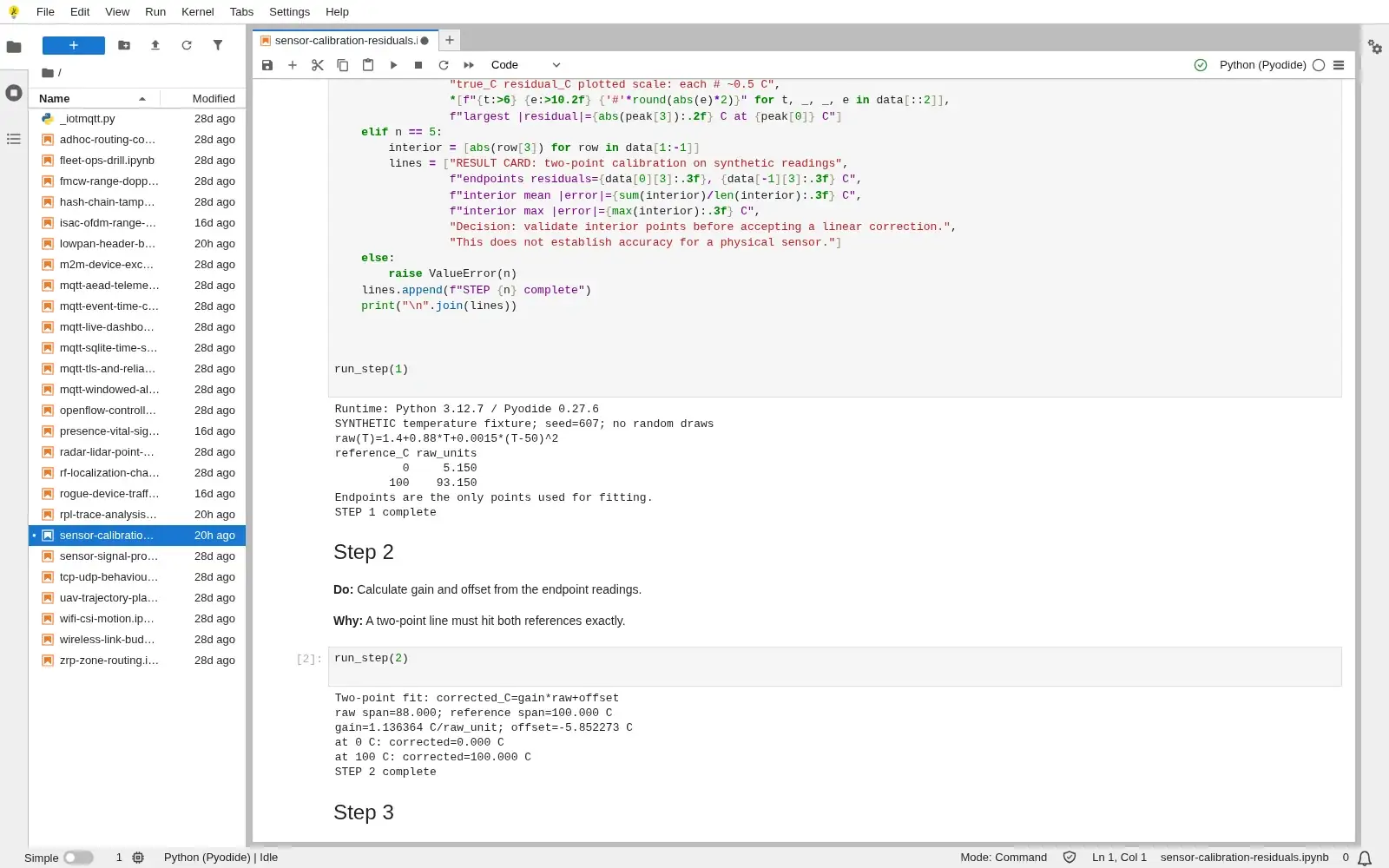
Step 1 · Python 3 in your browser (JupyterLite); numbered callout added to a real capture. Enlarge screenshot (new tab) Step 2
- Do
- In the JupyterLite notebook, run step 2 to fit gain and offset from the two endpoints.
- You will see
- Two-point fit: corrected_C=gain*raw+offset; raw span=88.000; reference span=100.000 C; gain=1.136364 C/raw_unit; offset=-5.852273 C
- Why it matters
- A linear fit must interpolate the two references exactly.
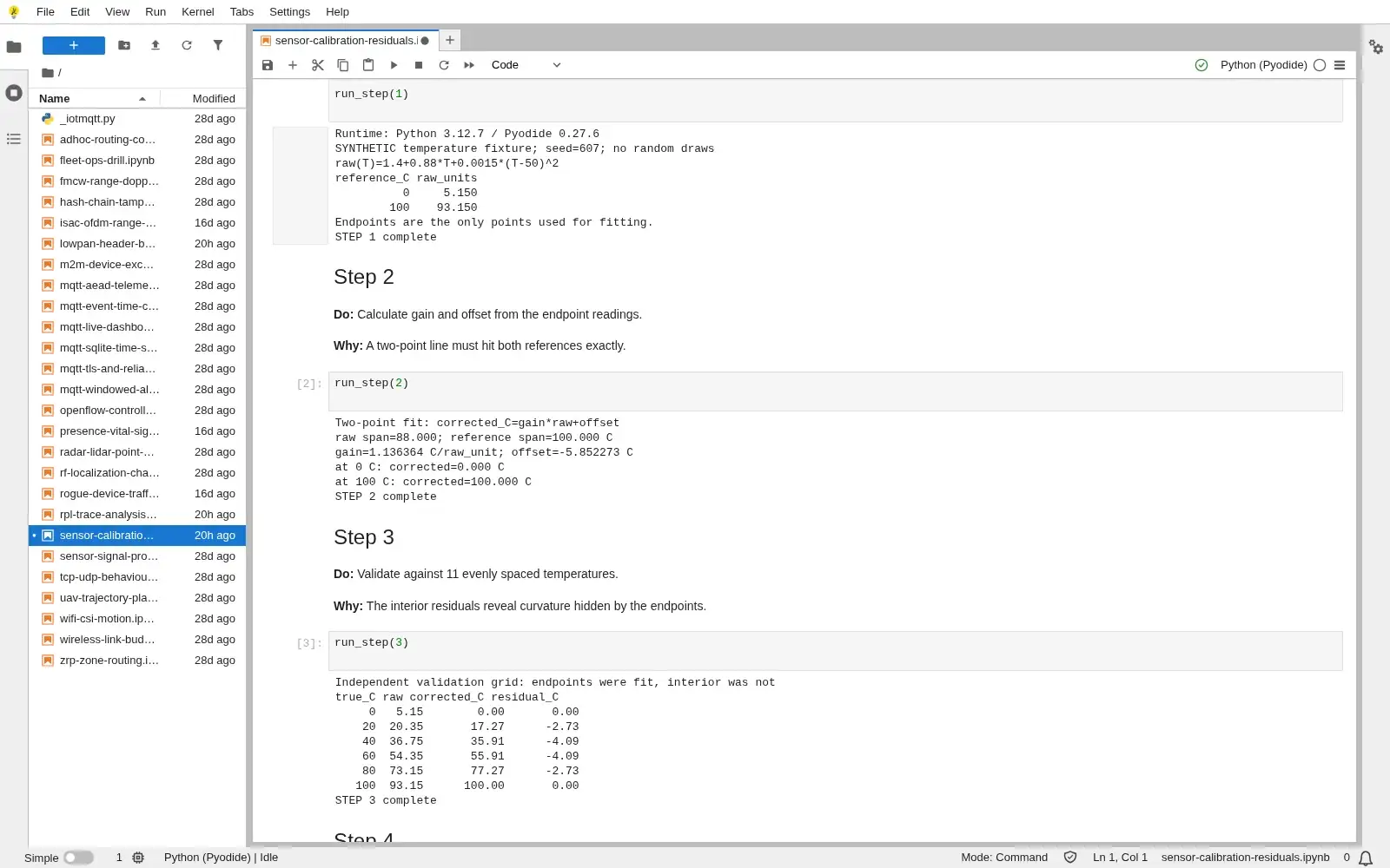
Step 2 · Python 3 in your browser (JupyterLite); numbered callout added to a real capture. Enlarge screenshot (new tab) Step 3
- Do
- In the JupyterLite notebook, run step 3 to test the corrected values across the span.
- You will see
- Independent validation grid: endpoints were fit, interior was not; true_C raw corrected_C residual_C; 0 5.15 0.00 0.00
- Why it matters
- Unused interior points test whether the line generalizes.
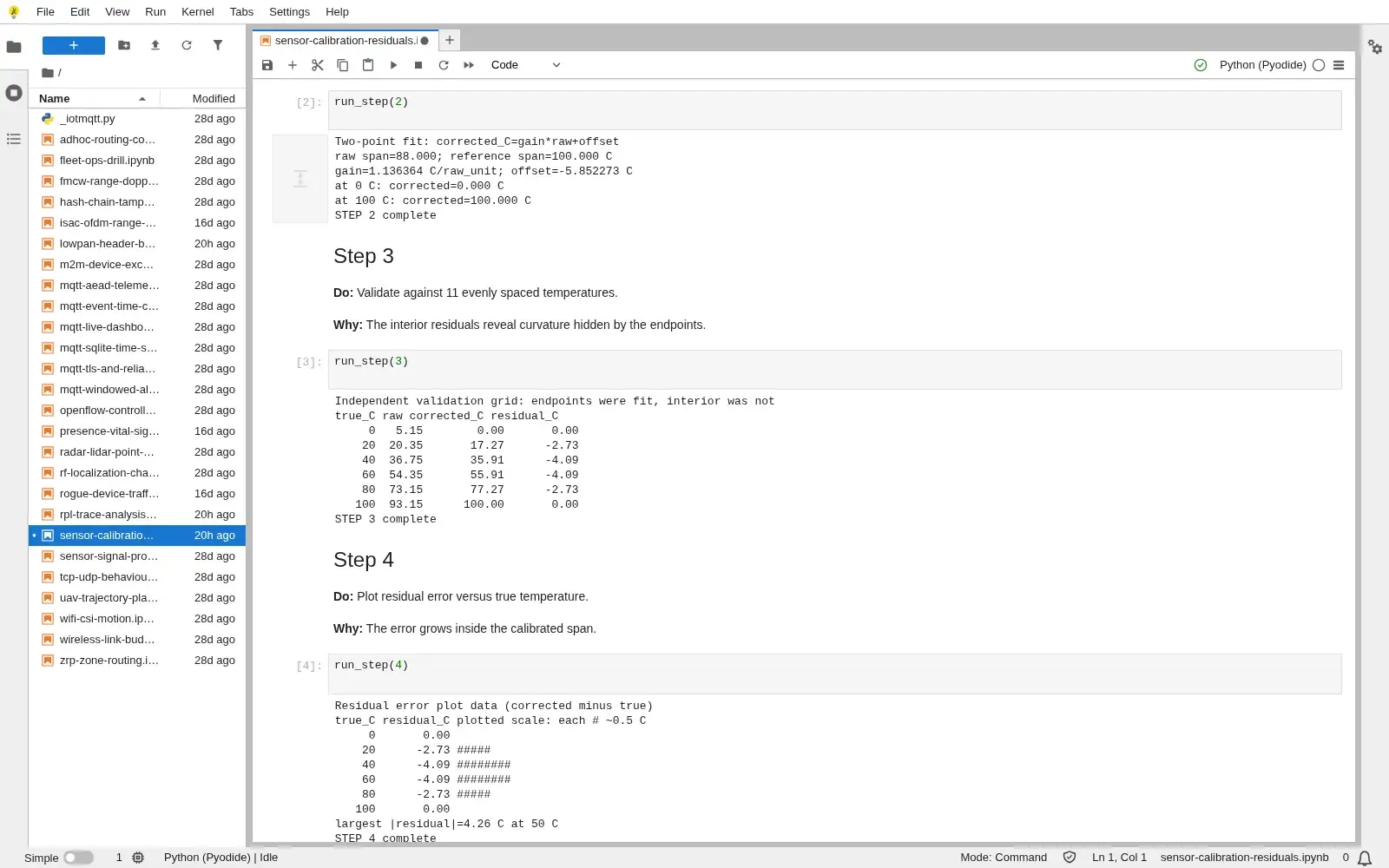
Step 3 · Python 3 in your browser (JupyterLite); numbered callout added to a real capture. Enlarge screenshot (new tab) Step 4
- Do
- In the JupyterLite notebook, run step 4 to plot residual error versus true temperature.
- You will see
- Residual error plot data (corrected minus true); true_C residual_C plotted scale: each # ~0.5 C; 0 0.00
- Why it matters
- A residual plot reveals curvature hidden by endpoint checks.
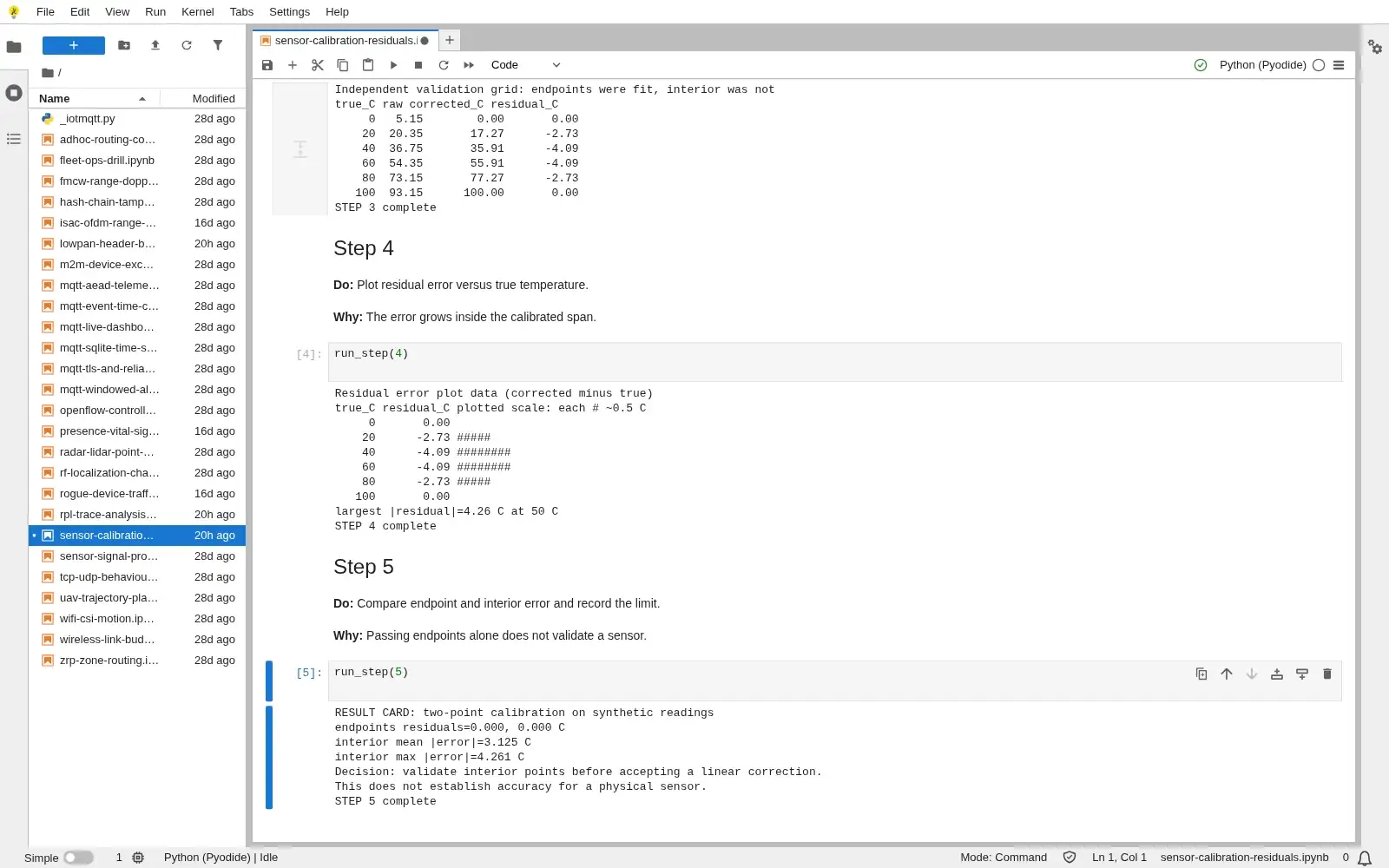
Step 4 · Python 3 in your browser (JupyterLite); numbered callout added to a real capture. Enlarge screenshot (new tab) Step 5
- Do
- In the JupyterLite notebook, run step 5 to compare interior and endpoint error.
- You will see
- RESULT CARD: two-point calibration on synthetic readings; endpoints residuals=0.000, 0.000 C; interior mean |error|=3.125 C
- Why it matters
- Span validation is required before accepting a correction.
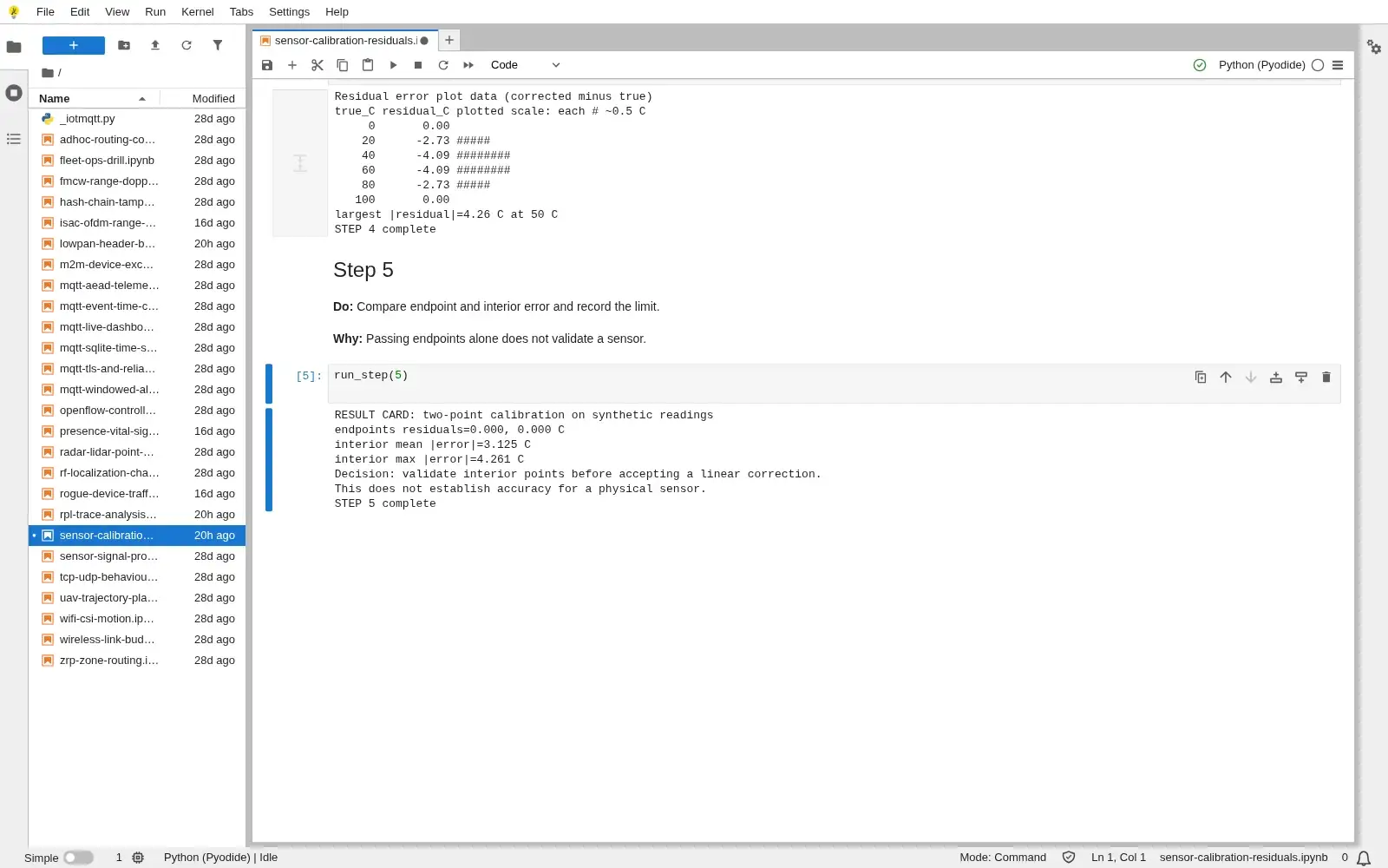
Step 5 · Python 3 in your browser (JupyterLite); numbered callout added to a real capture. Enlarge screenshot (new tab)
Chapter checks
These questions refer to the chapter’s examples. Use the return links to review their answers.
A sensor reads 20% when the true value is 10%, and reads 80% when the true value is 90%. What is the gain (slope) coefficient?
Return to the chapter’s knowledge checkYou need to calibrate a soil moisture sensor that will measure between 20% and 80% moisture in a greenhouse. Which reference points should you use?
Return to the chapter’s knowledge check
Return to Sensor Calibration: Math and Validation · Browse Labs