Sampling rate and aliased frequency
Explain how aliasing and anti-alias filters change sampled evidence.
Explain how aliasing and anti-alias filters change sampled evidence.
Predict the reading, then compare it with the measurement.
Python 3 in your browser (JupyterLite)
Python · no installExplain how aliasing and anti-alias filters change sampled evidence.
Open the notebook in your browser and run each Python cell; no install or account is needed.
Three ways to run: use JupyterLite here with no install; run main.py locally from the downloadable lab folder; or open the same notebook in Google Colab.
Steps
Step 1
- Do
- Run the Step 1 notebook cell to inspect the synthetic 7 Hz source and reference sample table.
- You will see
- SYNTHETIC sine fixture; seed=207; no random draws; source(t)=sin(2*pi*7 Hz*t); duration=1.000 s; reference time_s signal; 0.000 0.000; 0.025 0.891
- Why it matters
- The original generated signal fixes the source frequency before sampling.
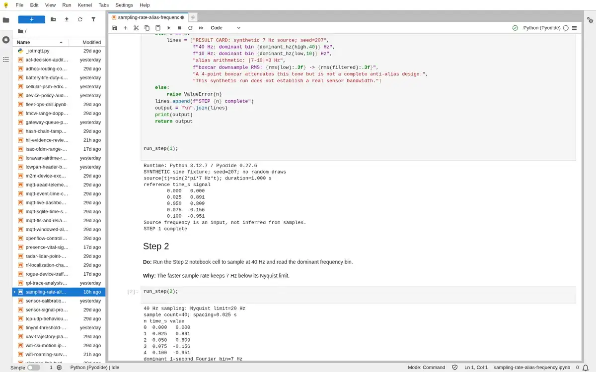
Step 1 · Python 3 in your browser (JupyterLite); numbered callout added to a real capture. Enlarge screenshot (new tab) Step 2
- Do
- Run the Step 2 notebook cell to sample at 40 Hz and read the dominant frequency bin.
- You will see
- 40 Hz sampling: Nyquist limit=20 Hz; sample count=40; spacing=0.025 s; dominant 1-second Fourier bin=7 Hz; inferred period=0.143 s
- Why it matters
- The faster sample rate keeps 7 Hz below its Nyquist limit.
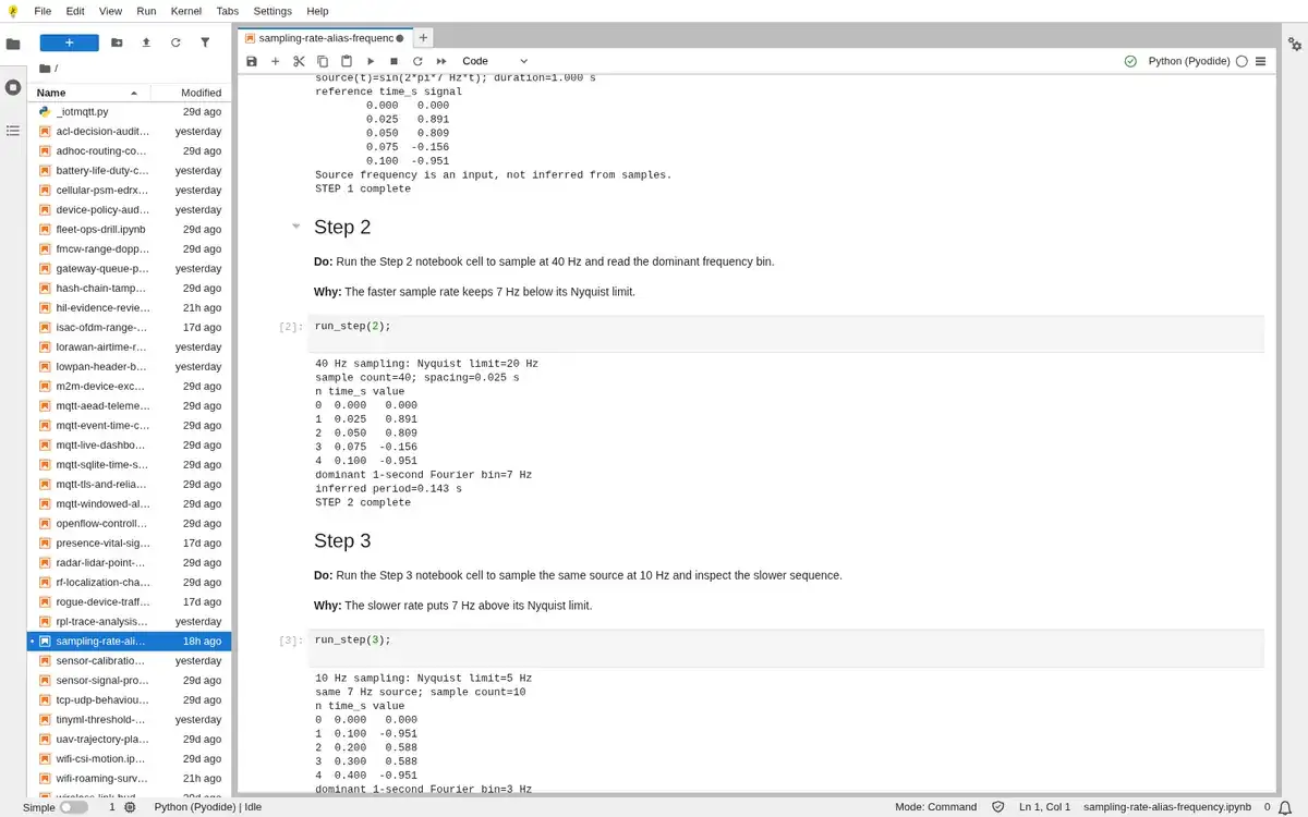
Step 2 · Python 3 in your browser (JupyterLite); numbered callout added to a real capture. Enlarge screenshot (new tab) Step 3
- Do
- Run the Step 3 notebook cell to sample the same source at 10 Hz and inspect the slower sequence.
- You will see
- 10 Hz sampling: Nyquist limit=5 Hz; same 7 Hz source; sample count=10; dominant 1-second Fourier bin=3 Hz; The visible sequence cycles more slowly.
- Why it matters
- The slower rate puts 7 Hz above its Nyquist limit.
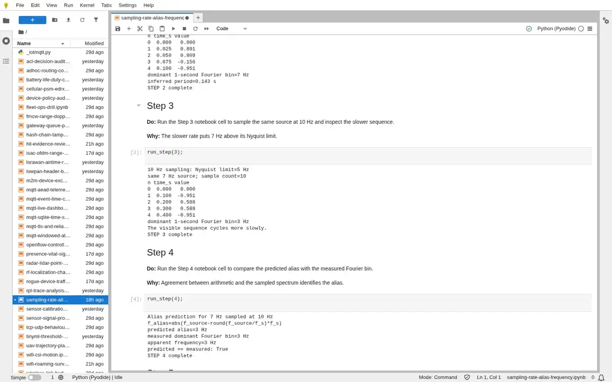
Step 3 · Python 3 in your browser (JupyterLite); numbered callout added to a real capture. Enlarge screenshot (new tab) Step 4
- Do
- Run the Step 4 notebook cell to compare the predicted alias with the measured Fourier bin.
- You will see
- Alias prediction for 7 Hz sampled at 10 Hz; f_alias=abs(f_source-round(f_source/f_s)*f_s); apparent frequency=3 Hz; predicted == measured: True
- Why it matters
- Agreement between arithmetic and the sampled spectrum identifies the alias.
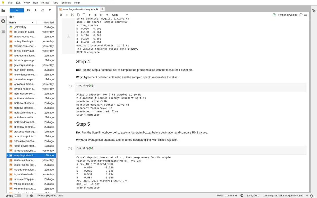
Step 4 · Python 3 in your browser (JupyterLite); numbered callout added to a real capture. Enlarge screenshot (new tab) Step 5
- Do
- Run the Step 5 notebook cell to apply a four-point boxcar before decimation and compare RMS values.
- You will see
- Causal 4-point boxcar at 40 Hz, then keep every fourth sample; filter output[n]=mean(high[4*n-k], k=0..3); raw RMS=0.707; filtered RMS=0.274; RMS ratio=0.387
- Why it matters
- An average can attenuate a tone before downsampling, with limited rejection.
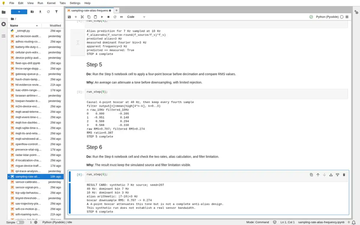
Step 5 · Python 3 in your browser (JupyterLite); numbered callout added to a real capture. Enlarge screenshot (new tab) Step 6
- Do
- Run the Step 6 notebook cell and check the two rates, alias calculation, and filter limitation.
- You will see
- RESULT CARD: synthetic 7 Hz source; seed=207; 40 Hz: dominant bin 7 Hz; A 4-point boxcar attenuates this tone but is not a complete anti-alias design.; This synthetic run does not establish a real sensor bandwidth.
- Why it matters
- The result must keep the simulated source and filter limitation visible.
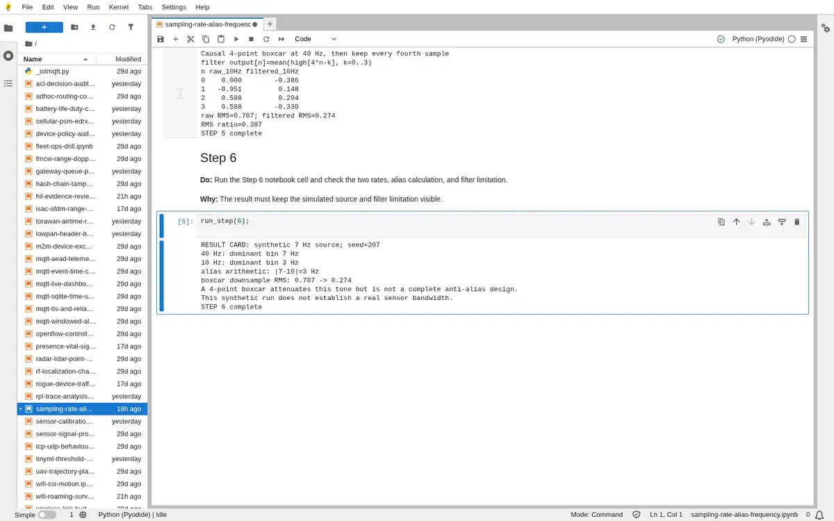
Step 6 · Python 3 in your browser (JupyterLite); numbered callout added to a real capture. Enlarge screenshot (new tab)
Chapter checks
These questions refer to the chapter’s examples. Use the return links to review their answers.
You need to sample a 500 Hz signal. What is the minimum sampling rate according to Nyquist?
Return to the chapter’s knowledge checkAn ADC samples at eight kilohertz and the wanted signal ends at one kilohertz. Which anti-alias filter plan is reviewable?
Return to the chapter’s knowledge check
Return to Sampling and Aliasing: Nyquist and Filters · Browse Labs