Residual score for sensor anomalies
Compute a residual score while keeping drift and alert limits visible.

Compute a residual score while keeping drift and alert limits visible.
Predict the reading, then compare it with the measurement.
Python 3 in your browser (JupyterLite)
Python · no installCompute a residual score while keeping drift and alert limits visible.
Open the notebook in your browser and run each Python cell; no install or account is needed.
Three ways to run: use JupyterLite here with no install; run main.py locally from the downloadable lab folder; or open the same notebook in Google Colab.
Steps
Step 1
- Do
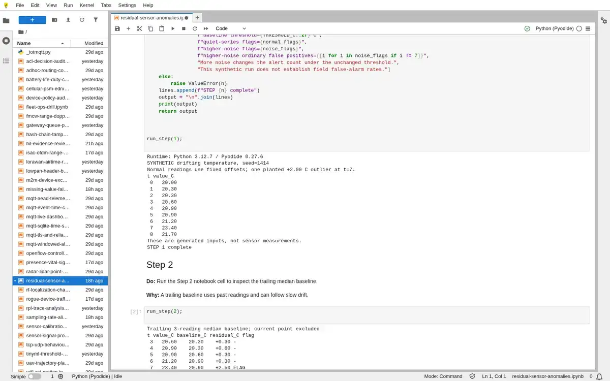
- Run the Step 1 notebook cell and inspect the drifting synthetic series with its planted outlier.
- You will see
- SYNTHETIC drifting temperature, seed=1414; Normal readings use fixed offsets; one planted +2.00 C outlier at t=7.; t value_C; 0 20.00; 1 20.30
- Why it matters
- The known planted event permits a direct check of detector behavior.
Step 1 · Python 3 in your browser (JupyterLite); numbered callout added to a real capture. Enlarge screenshot (new tab) Step 2
- Do
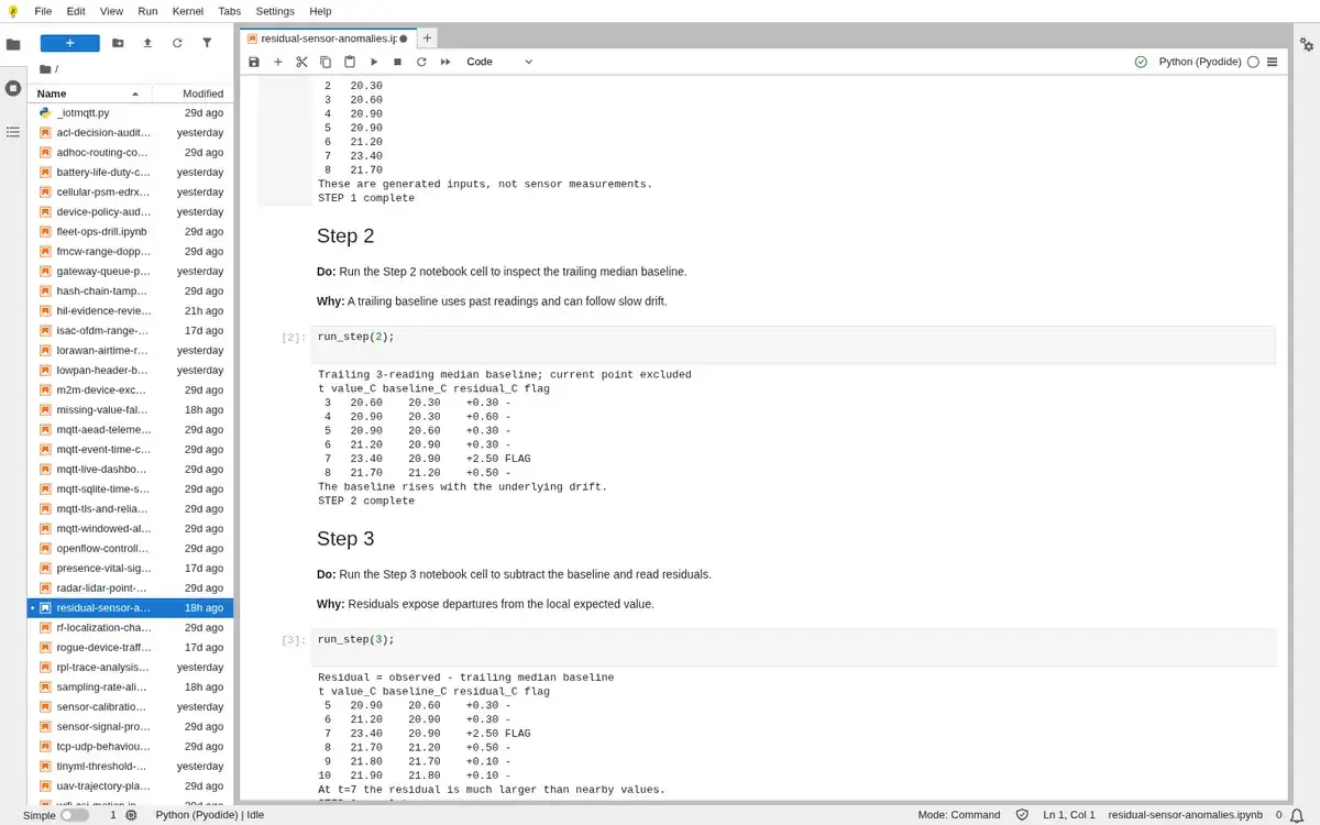
- Run the Step 2 notebook cell to inspect the trailing median baseline.
- You will see
- Trailing 3-reading median baseline; current point excluded; t value_C baseline_C residual_C flag; 8 21.70 21.20 +0.50 -; The baseline rises with the underlying drift.
- Why it matters
- A trailing baseline uses past readings and can follow slow drift.
Step 2 · Python 3 in your browser (JupyterLite); numbered callout added to a real capture. Enlarge screenshot (new tab) Step 3
- Do
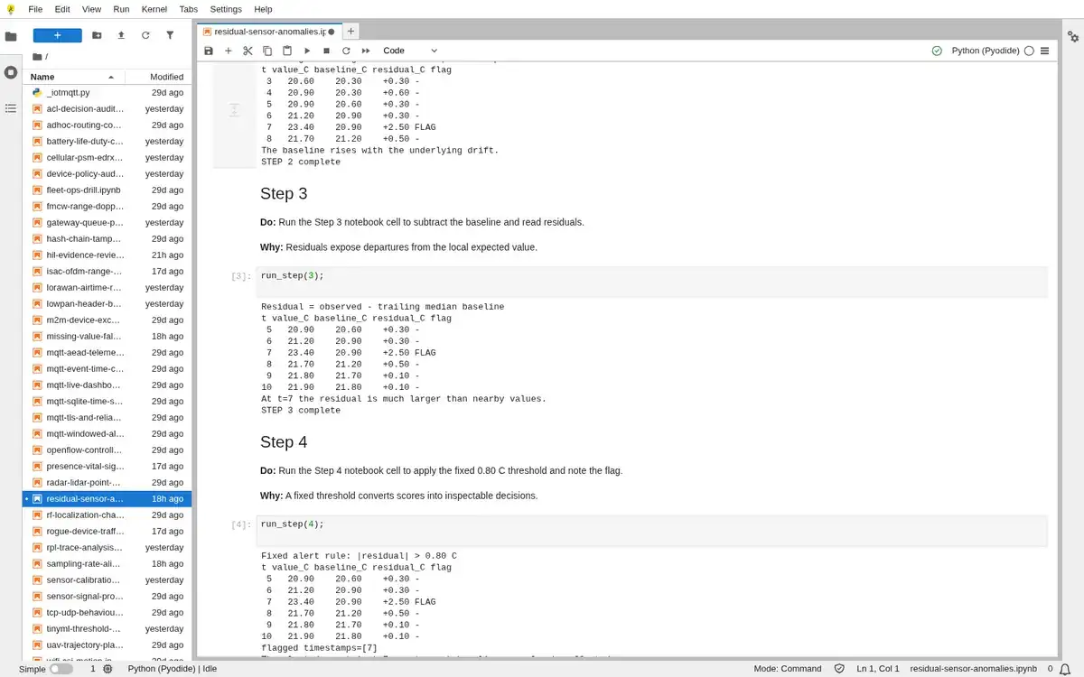
- Run the Step 3 notebook cell to subtract the baseline and read residuals.
- You will see
- Residual = observed - trailing median baseline; t value_C baseline_C residual_C flag; 10 21.90 21.80 +0.10 -; At t=7 the residual is much larger than nearby values.
- Why it matters
- Residuals expose departures from the local expected value.
Step 3 · Python 3 in your browser (JupyterLite); numbered callout added to a real capture. Enlarge screenshot (new tab) Step 4
- Do
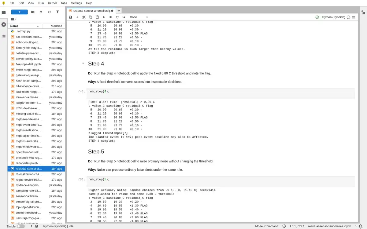
- Run the Step 4 notebook cell to apply the fixed 0.80 C threshold and note the flag.
- You will see
- Fixed alert rule: |residual| > 0.80 C; t value_C baseline_C residual_C flag; flagged timestamps=[7]; The planted event is t=7; post-event baseline may also be affected.
- Why it matters
- A fixed threshold converts scores into inspectable decisions.
Step 4 · Python 3 in your browser (JupyterLite); numbered callout added to a real capture. Enlarge screenshot (new tab) Step 5
- Do
- Run the Step 5 notebook cell to raise ordinary noise without changing the threshold.
- You will see
- Higher ordinary noise: random choices from -1.10, 0, +1.10 C; seed=1414; same planted t=7 value and same 0.80 C threshold; 9 21.80 22.30 -0.50 -; flagged timestamps=[4, 6, 7, 8]
- Why it matters
- Noise can produce ordinary false alerts under the same rule.
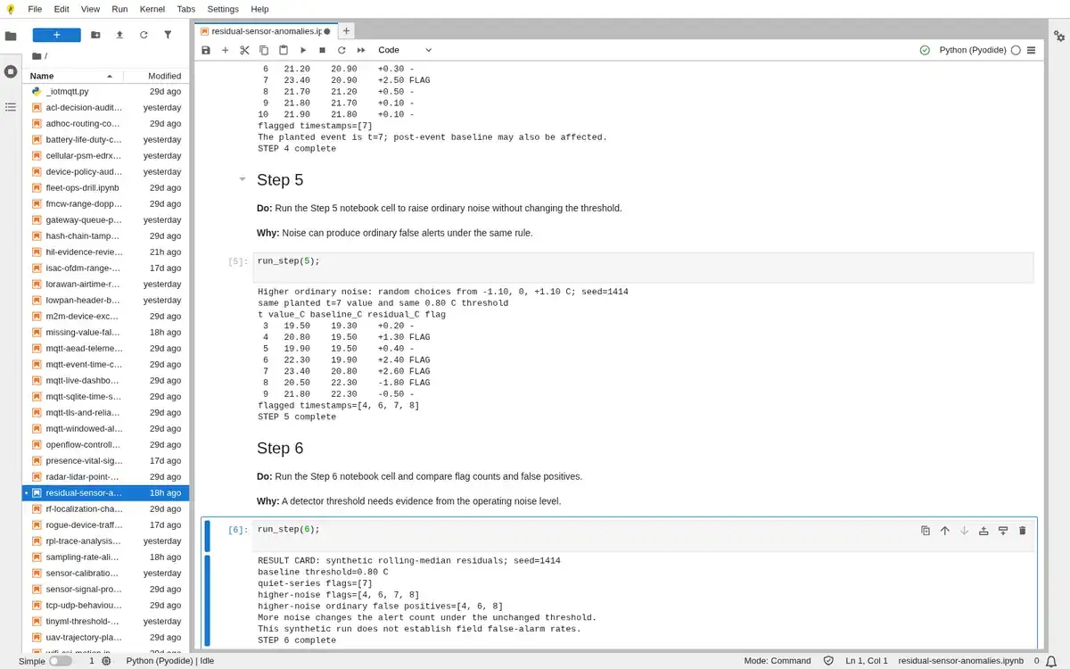
Step 5 · Python 3 in your browser (JupyterLite); numbered callout added to a real capture. Enlarge screenshot (new tab) Step 6
- Do
- Run the Step 6 notebook cell and compare flag counts and false positives.
- You will see
- RESULT CARD: synthetic rolling-median residuals; seed=1414; baseline threshold=0.80 C; More noise changes the alert count under the unchanged threshold.; This synthetic run does not establish field false-alarm rates.
- Why it matters
- A detector threshold needs evidence from the operating noise level.
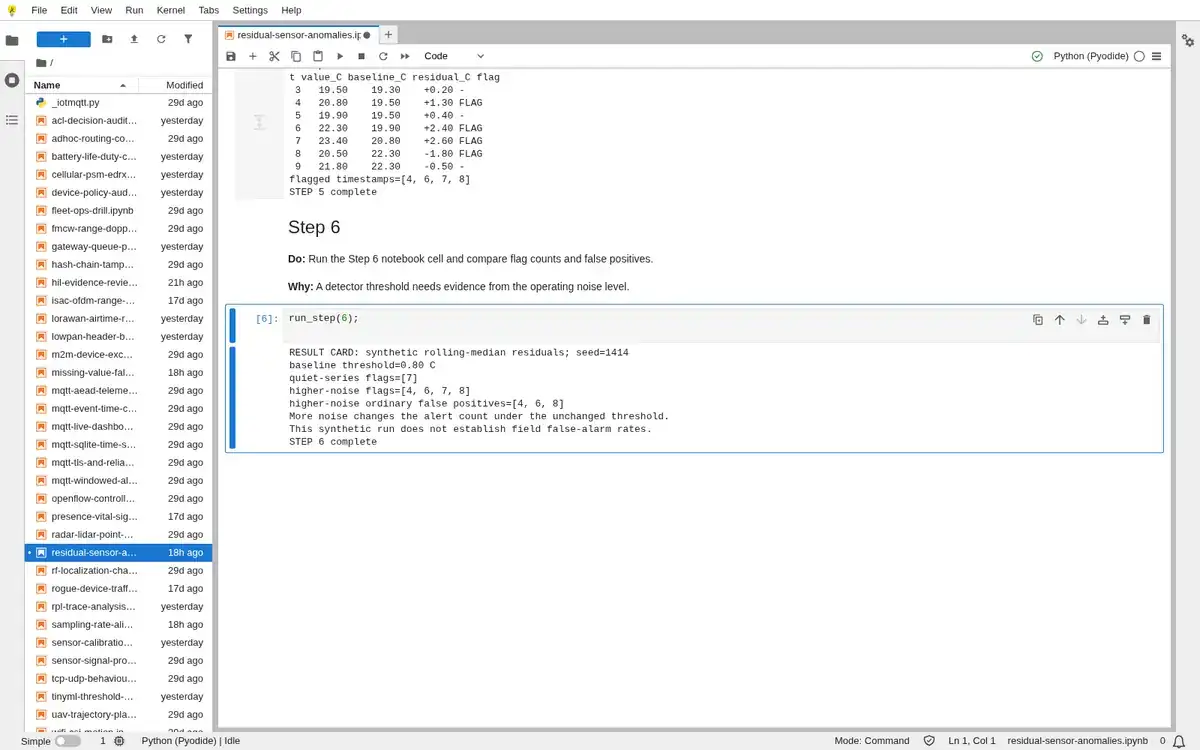
Step 6 · Python 3 in your browser (JupyterLite); numbered callout added to a real capture. Enlarge screenshot (new tab)
Chapter checks
These questions refer to the chapter’s examples. Use the return links to review their answers.
Why should a seasonal IoT signal usually be scored on residuals instead of raw readings?
Return to the chapter’s knowledge checkThe matching seasonal baseline is 18 kW and the observed load is 31 kW. The alert band is ±4 kW, but the reading arrived 2 minutes after a 1-minute action deadline. What is the defensible result?
Return to the chapter’s knowledge check
Return to Time-Series Anomalies: Baselines and Residuals · Browse Labs