Reuse a synthetic OFDM frame for range evidence
Transform a known OFDM frame into a synthetic delay profile and justify one sensing-airtime and payload operating point.

Radio Remi: predict first, inspect every intermediate value, and keep the claim inside the evidence.
Predict the reading, then compare it with the measurement.
Python 3 in your browser (JupyterLite)
Python · no installTransform a known OFDM frame into a synthetic delay profile and justify one sensing-airtime and payload operating point.
Open the notebook in your browser and run each Python cell; no install or account is needed.
Three ways to run: use JupyterLite here with no install; run main.py locally from the downloadable lab folder; or open the same notebook in Google Colab.
Steps
Step 1
- Do
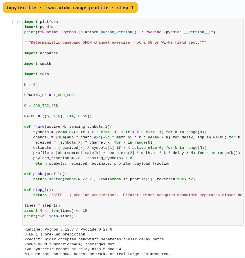
- Predict what narrower occupied bandwidth will do to two echoes.
- You will see
- The known tones, frequency spacing, echo delay bins, and synthetic status print.
- Why it matters
- Wider occupied bandwidth improves the ability to separate nearby delays; longer coherent observation improves Doppler resolution but slows the result and demands more stable timing.
Step 1 · Python 3 in your browser (JupyterLite); numbered callout added to a real capture. Enlarge screenshot (new tab) Step 2
- Do
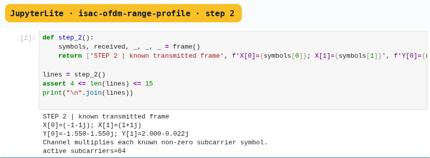
- Generate the known OFDM symbols and received values.
- You will see
- Two transmitted and two received complex values print.
- Why it matters
- An OFDM transmitter places known or decodable symbols $X[k]$ on many subcarriers.
Step 2 · Python 3 in your browser (JupyterLite); numbered callout added to a real capture. Enlarge screenshot (new tab) Step 3
- Do
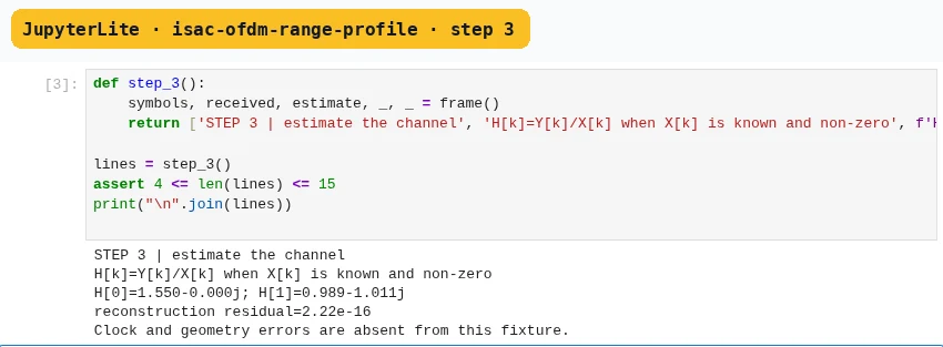
- Divide received values by known non-zero symbols.
- You will see
- Two channel estimates and the reconstruction residual print.
- Why it matters
- Where $X[k]$ is known and non-zero, the channel estimate is $H[k]=Y[k]/X[k]$.
Step 3 · Python 3 in your browser (JupyterLite); numbered callout added to a real capture. Enlarge screenshot (new tab) Step 4
- Do
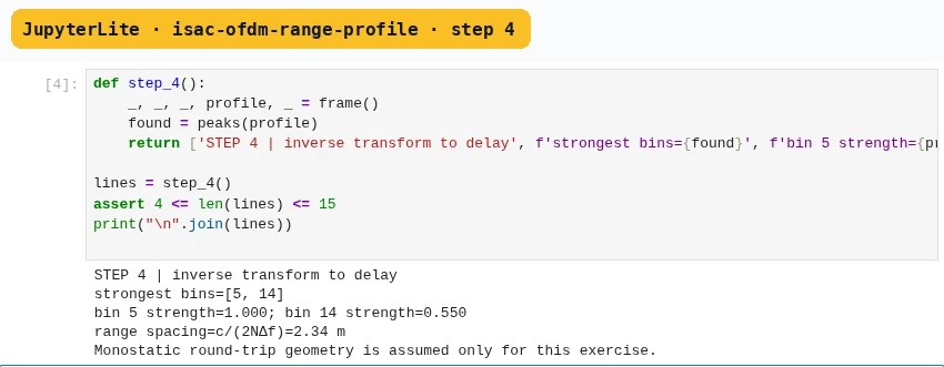
- Transform the channel estimate into a delay profile.
- You will see
- Two strongest bins, peak strengths, and round-trip range-bin spacing print.
- Why it matters
- An inverse Fourier transform across subcarriers turns frequency variation into a delay profile.
Step 4 · Python 3 in your browser (JupyterLite); numbered callout added to a real capture. Enlarge screenshot (new tab) Step 5
- Do
- Compare full and narrow occupied bandwidth.
- You will see
- Four quantitative resolution and peak-shape values print.
- Why it matters
- More bandwidth can separate closer reflectors, but spectrum availability, radio front ends, channel occupancy, and regulations constrain it.
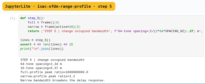
Step 5 · Python 3 in your browser (JupyterLite); numbered callout added to a real capture. Enlarge screenshot (new tab) Step 6
- Do
- Vary sensing slots inside an eight-symbol schedule.
- You will see
- A four-row table reports the modeled payload fraction.
- Why it matters
- Data symbols, pilots, guard intervals, retransmissions, beams, and sensing bursts all compete for finite resources.
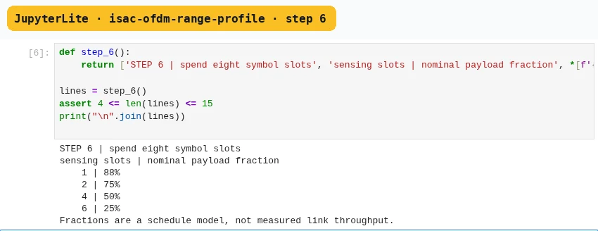
Step 6 · Python 3 in your browser (JupyterLite); numbered callout added to a real capture. Enlarge screenshot (new tab) Step 7
- Do
- Write a bounded operating-point result card.
- You will see
- The selected and rejected schedules print with untested field requirements.
- Why it matters
- Report payload throughput, packet delay, packet loss, range-bin spacing, update interval, false alarms, missed detections, energy, and compute load separately.
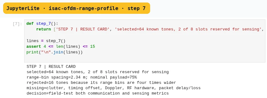
Step 7 · Python 3 in your browser (JupyterLite); numbered callout added to a real capture. Enlarge screenshot (new tab)
Chapter checks
These questions refer to the chapter’s examples. Use the return links to review their answers.
Why must the receiver know or decode an OFDM symbol before using Y[k]/X[k] as a channel estimate?
Return to the chapter’s knowledge checkWhat proves a chosen ISAC schedule?
Return to the chapter’s knowledge check
Return to Integrated Sensing and Communication for IoT · Browse Labs