Public-sector smart-city platform, Sentilo, and civic outcomes
Current
Volkswagen Predictive Maintenance and Cross-Case Lessons
Industrial predictive maintenance, ROI, and the cross-case framework
25.1 VW Maintenance Prediction
25.2 Volkswagen Background and Challenge
Volkswagen’s Wolfsburg plant, the largest automobile manufacturing facility globally, produces 3,800 vehicles daily using 7,500 robots and 44,000 employees. Unplanned downtime from equipment failures costs $1.3 million per hour in lost production. Traditional reactive maintenance led to unexpected breakdowns, while preventive maintenance on fixed schedules wasted resources replacing components with remaining useful life.
See how IoT transforms manufacturing through predictive maintenance and smart factories.
Key Challenges:
7,500+ robots across 68 production lines creating massive data volumes
Downtime cascades affecting entire production line (domino effect)
Legacy equipment (10-20 years old) lacking modern sensor capabilities
Heterogeneous equipment from 50+ vendors with incompatible protocols
Need to retrofit IoT without disrupting 24/7 production
ROI pressure: Investment must pay back within 18 months
25.3 Volkswagen Solution Architecture
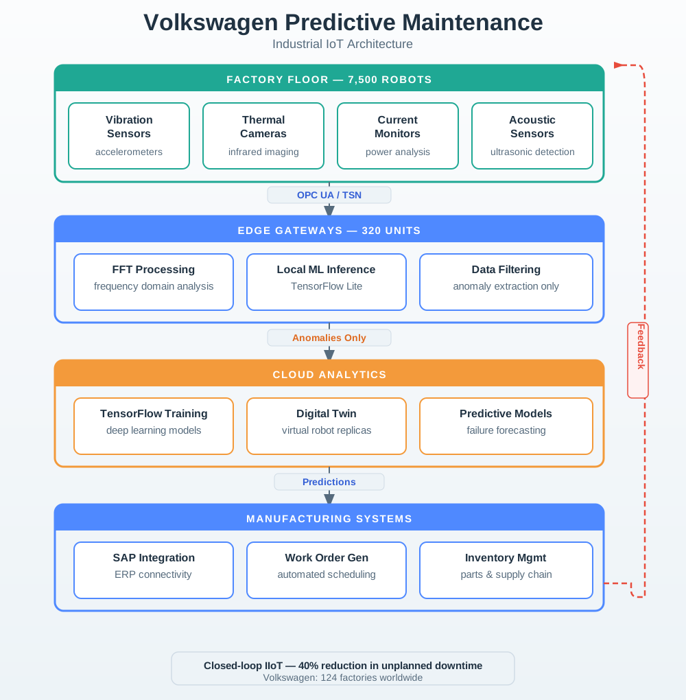
Volkswagen partnered with Siemens to implement a comprehensive Industrial IoT (IIoT) predictive maintenance system integrating edge computing, machine learning, and existing manufacturing execution systems (MES).
Collected baseline data and trained initial models
Phase 2: Model Development (6 months)
Collected 180TB of operational data
Labeled failure events from maintenance logs (250 failures)
Trained LSTM neural networks for time-series anomaly detection
Achieved 87% accuracy in predicting failures 48 hours in advance
Reduced false positive rate to <5%
Phase 3: Plant-Wide Rollout (18 months)
Retrofitted 7,500 robots and critical equipment
Deployed 320 edge gateways across 68 production lines
Integrated with SAP MES for automated work order creation
Trained maintenance staff on new predictive alerts
Technical Innovations:
Edge Processing Strategy:
FFT (Fast Fourier Transform) on edge gateways to extract frequency domain features
Local anomaly detection models (TensorFlow Lite) running inference every 100ms
Only anomalies and aggregated statistics sent to cloud (99.8% data reduction)
72-hour local buffer for offline operation during network issues
Multi-Modal Sensor Fusion:
Combined vibration, thermal, acoustic, and current data
Improved accuracy from 72% (single sensor) to 87% (sensor fusion)
Different sensors detect different failure modes (bearings vs. motors vs. pneumatics)
Digital Twin Integration:
Virtual model of production line simulates impact of taking equipment offline
Optimizes maintenance scheduling to minimize production disruption
Simulates “what-if” scenarios for maintenance strategies
Phoebe’s Field Notes: How A Bearing Vibration Becomes A Voltage
Phoebe’s Why
The MEMS accelerometers on Volkswagen’s robots do not measure acceleration directly – nothing electrical can. They measure a change in capacitance and invert a known equation to report acceleration. A tiny proof mass hangs on springs between two fixed plates, forming two capacitors back to back. Bearing vibration is a force, and force moves the mass a few tens of nanometres against the springs. That nanometre-scale motion changes the gap in each capacitor, which is the only electrical property the chip can actually sense. Everything downstream – the amplifier, the ADC, the g-value in the log file – is that displacement’s capacitance change wearing a unit conversion.
The Derivation
Newton’s second law and Hooke’s law fix the proof mass’s displacement under acceleration \(a\):
\[F = ma = kx \;\Rightarrow\; x = \frac{ma}{k}\]
Each parallel-plate capacitor follows \(C = \varepsilon_0 A/d\); for a differential pair with gap \(d_0\) closing on one side and opening on the other by \(x\), the small-signal difference is
\[\Delta C = C_1 - C_2 \approx \frac{2\varepsilon_0 A}{d_0^2}\,x\]
A charge amplifier with feedback capacitance \(C_f\) and excitation \(V_{ref}\) turns that into a voltage the ADC can hold:
\[V_{out} = \frac{\Delta C}{C_f}\,V_{ref}\]
The reading is used by inverting the whole chain: measured \(V_{out}\) gives \(\Delta C\), \(\Delta C\) gives \(x\), and \(x = ma/k\) gives the acceleration the model actually trains on.
Worked Numbers: One 5g Bearing Event
The chapter names no die geometry, so take catalog-typical IIoT-grade MEMS figures: plate area \(A = 0.400\ \mathrm{mm}^2\), gap \(d_0 = 2.00\ \mu\)m, a \(5.00\) kHz mechanical resonance, and a \(1.00\times10^{-10}\) kg proof mass.
Base capacitance: \(C_0 = \varepsilon_0 A/d_0 = 1.77\) pF; spring constant from resonance, \(k = m(2\pi\times5000)^2 = 0.0987\) N/m
At a \(5g\) (\(49.1\ \mathrm{m/s^2}\)) bearing-defect event: \(F = ma = 4.91\times10^{-9}\) N, so \(x = F/k = 49.7\) nm – a nanometre-scale motion, which is exactly why capacitance sensing, not a strain gauge, is used here
With \(C_f = 1.00\) pF and \(V_{ref} = 1.00\) V: \(V_{out} = (88.0\ \mathrm{fF}/1.00\ \mathrm{pF})\times1.00\ \mathrm{V} = 88.0\) mV, a sensitivity of \(17.6\) mV/g – the same order of magnitude as published IIoT accelerometer datasheets, a useful sanity check on the assumptions
That inversion chain – voltage to capacitance to displacement to force to acceleration – is also why this chapter’s multi-modal fusion helps: the thermal, acoustic, and current sensors each invert a different governing equation (radiated power, sound pressure, resistive heating), so they do not share the same blind spots. A bearing fault that barely moves the proof mass can still show up as heat or current draw, which is a real, physical reason multi-sensor fusion raised accuracy from 72% to 87% in this chapter’s own numbers, not just a modeling trick.
25.6 Predictive Maintenance Decision Pipeline
The following diagram illustrates how sensor data flows through Volkswagen’s predictive maintenance system, from raw measurement to maintenance action:
Step 1
Sensing
Robots stream vibration, thermal, acoustic, and current data from the shop floor.
Step 2
Edge Feature Extraction
Gateways run FFT and windowing every few seconds to compress raw waveforms into health indicators.
Step 3
Anomaly Scoring
TensorFlow Lite models combine the sensor channels and estimate severity plus time-to-failure.
Step 4
Workflow Decision
Low-risk cases keep monitoring, medium-risk cases schedule maintenance, and severe cases trigger immediate alerts.
Step 5
Action in MES
Approved alerts create work orders, reserve spare parts, and update the digital twin for scheduling.
25.7 Volkswagen Results and Impact
Quantified Outcomes:
Operational Improvements:
Unplanned Downtime: Reduced by 42% (from 85 hours/month to 49 hours/month)
Maintenance Costs: Reduced by 28% ($12.4M to $8.9M annually)
Equipment Lifespan: Extended by 18% through optimal maintenance timing
Spare Parts Inventory: Reduced by 35% through predictive ordering
Maintenance Staff Productivity: +32% through targeted interventions
Financial Impact:
Annual Cost Savings: $47 million
Reduced downtime: $28M (42% reduction x $1.3M/hour x 49 hours saved/month)
Lower maintenance costs: $3.5M (preventive to predictive shift)
Spare parts optimization: $8.2M (inventory reduction)
Extended equipment life: $7.3M (deferred capital expenditure)
Project Investment: $23 million
Payback Period: 7 months (vs. target of 18 months)
5-Year ROI: 912%
25.8 Putting Numbers to It
Volkswagen’s 7-month payback comes from dividing the $23M investment by monthly savings: $23M / ($47M per year / 12) = about 5.9 months. The 5-year ROI calculation is (($47M x 5) - $23M) / $23M x 100%, or about 912%. Worked example: Over 60 months, system generates $235M in savings against $23M investment. The non-intuitive insight: downtime cost dominates at $1.3M/hour. Preventing just 18 hours of unplanned downtime annually pays for the entire $23M system. This explains why predictive maintenance achieves payback 2.5x faster than Volkswagen’s 18-month target.
Beyond the obvious production loss, downtime includes:
Cost Category
Typical % of Total
Example
Lost production value
50-60%
Vehicles not built, products not shipped
Emergency labor (overtime)
10-15%
Weekend call-ins, contractor premiums
Expedited spare parts
5-10%
Air freight for critical components
Scrap and rework
5-15%
Partially completed products, quality issues
Cascading effects
10-20%
Downstream lines waiting, supplier penalties
Customer penalties
Variable
Late delivery fines, lost future orders
25.17 Predictive Maintenance Savings
Formula:
Annual Savings = (Current Downtime Hours x Hourly Cost x % Reduction) +
                 (Current Maintenance Cost x % Reduction) +
                 (Spare Parts Inventory x Carrying Cost x % Reduction)
Example (Volkswagen-scale):
Current downtime: 85 hours/month x $1.3M = $110.5M/year
Downtime reduction: 42% = $46.4M saved
Current maintenance: $12.4M/year
Maintenance reduction: 28% = $3.5M saved
Spare parts inventory: $24M x 15% carrying cost = $3.6M/year
Inventory reduction: 35% x $3.6M = $1.3M saved
Total annual savings: $51.2M
25.18 Typical ROI by Implementation Approach
Approach
Investment
Accuracy
Payback
5-Year ROI
Threshold alerts only
Low ($50K)
40-60%
6-12 mo
200-400%
ML on single sensor type
Medium ($200K)
70-80%
12-18 mo
400-600%
Multi-sensor fusion + edge ML
High ($1M+)
85-95%
6-12 mo
800-1200%
Full digital twin integration
Very High ($5M+)
90-98%
12-24 mo
600-1000%
Key Insight: The highest investment approach (multi-sensor fusion + edge ML) often has the shortest payback because the accuracy improvement dramatically reduces false positives and catches more actual failures.
Checkpoint: ROI Arithmetic
You now know which numbers make predictive maintenance persuasive:
Volkswagen invested $23M and reports $47M in annual savings, giving a 7-month payback.
At $1.3M/hour, preventing just 18 hours of unplanned downtime annually can pay for the system.
The five-year view compares $235M in savings against $23M investment for about 912% ROI.
25.19 Predictive Maintenance Savings
Calculate total savings from implementing predictive maintenance across multiple benefit categories.
Understanding how deployment strategies differ across domains helps practitioners select the right approach for their context.
Deployment rhythm
Rollout speed follows the environment
Cities scale through visible public-service phases, while factories scale through controlled pilots and rapid replication.
Data architecture
Openness versus latency
Barcelona optimized for shared civic data and APIs. Volkswagen optimized for local edge decisions and deterministic industrial networking.
Human adoption
Trust gates both projects
Citizens, city departments, and startups had to buy into Barcelona’s platform; technicians had to trust Volkswagen’s alerts.
Economic proof
ROI must be legible early
Barcelona used visible service savings to fund expansion, while Volkswagen used short payback on critical lines to justify plant-wide rollout.
25.21 Side-by-Side Analysis
Dimension
Barcelona Smart City
Volkswagen IIoT
Deployment Model
Multi-year phased rollout (3 phases over 8 years)
Rapid pilot-to-scale (21 months total)
Data Strategy
Cloud-centric, open data APIs
Edge-first, 99.8% processed locally
Platform Philosophy
Open-source (Sentilo), vendor-neutral
Vendor partnership (Siemens), purpose-built
Primary Network
City-owned 500km fiber + LoRaWAN
OPC UA over TSN (deterministic)
Integration Challenge
20+ departments, legacy city systems
50+ equipment vendors, heterogeneous protocols
Success Metric
Annual savings ($232M) + economic impact ($2.6B)
Payback period (7 months) + ROI (912%)
Change Management
Citizen engagement + developer ecosystem
Technician trust-building via parallel operation
Data Quality Issue
Sensor calibration across outdoor environments
Incomplete maintenance logs (40% missing data)
Scale Challenge
Geographic distribution across urban area
Temporal: 85TB/day from 30,000 sensors
Privacy Concern
Citizen surveillance, GDPR compliance
Proprietary manufacturing process data
25.22 Transferable Lessons
Both case studies, despite operating in very different domains, converge on these universal principles:
Start small, prove value, then scale – Barcelona began in the 22@ innovation district; Volkswagen started with 150 robots on one production line
Infrastructure investment precedes application value – Barcelona invested in fiber; Volkswagen invested in edge gateways
User adoption determines success more than technology – Barcelona needed citizen and developer engagement; Volkswagen needed technician trust
Data quality trumps data quantity – Barcelona’s open data required calibration; Volkswagen’s curated 3-month dataset outperformed 6 months of uncurated data
Budget for the “invisible” work – Both projects found integration and change management consumed 40-50% of effort
25.23 Enterprise IoT Pitfalls
25.23.1 Case Study Pitfalls
Pitfall 1: Technology-First Thinking Teams select sensors and platforms before understanding the workflow they need to improve. Both Barcelona and Volkswagen succeeded because they started with the problem (city inefficiency, equipment downtime), not the technology.
Pitfall 2: Ignoring the “Last Mile” of User Adoption A technically perfect system fails if users do not trust or use it. Volkswagen learned this painfully: 18% false positive rates caused technicians to ignore life-saving alerts. Always measure and optimize for the human in the loop.
Pitfall 3: Underestimating Integration Costs Barcelona spent 40% of implementation effort on integrating 20+ legacy systems. Many IoT budgets allocate 80% to hardware and software, leaving insufficient resources for the integration “glue” that makes systems work together.
Pitfall 4: Planning for Deployment Without Planning for Maintenance Sensor lifespan varies from 3-7 years. Without a replacement and maintenance budget (10-15% annually), a thriving IoT system decays into an expensive collection of dead sensors within 5 years.
Pitfall 5: All-or-Nothing Deployment Both case studies used phased deployment with quick-win pilots. Organizations that attempt city-wide or plant-wide deployment in a single phase face higher risk of failure and loss of stakeholder confidence.
Checkpoint: Transfer Risks
You now know what to protect when adapting either case:
Barcelona warns that integration across 20+ departments can consume 40% of implementation effort.
Volkswagen warns that a technically strong system can still fail when an 18% false positive rate erodes trust.
Both cases favor bounded pilots, visible early results, and maintenance budgets of 10-15% annually.
25.24 Knowledge Check: Cross-Case Analysis
25.25 Case Study Lessons Framework
Use this framework when designing your own IoT deployment, drawing from the patterns observed in both case studies:
1
Problem Definition
Quantify where downtime, waste, energy cost, or service friction is highest before selecting technology.
2
Pilot Design
Choose a bounded, high-impact pilot with measurable success metrics and a short review loop.
3
Quick Win Execution
Deliver visible savings fast enough to secure funding, operational trust, and organizational air cover.
4
Data & ML Maturation
Improve labels, calibration, and false-positive performance until the system supports real workflow decisions.
5
Scale-Out
Standardize deployment patterns, use pilot savings to fund rollout, and avoid all-at-once expansion.
6
Ecosystem Growth
Open APIs, partner processes, and feedback loops convert a successful pilot into a durable platform.
Phase-by-Phase Guidance:
Phase
Key Actions
Case Study Evidence
1. Problem Definition
Quantify current costs (downtime, waste, energy); identify Pareto distribution of impact
VW: 20% of equipment caused 80% of downtime; Barcelona: water and energy were largest cost centers
2. Pilot Design
Select highest-impact area; define success metrics; set 6-month timeline
VW: 150 robots on Body Shop Line 3; Barcelona: 22@ innovation district
Barcelona’s open-source Sentilo enabled 1,200+ startups and 47,000 jobs through API access
False Positive Reduction
User Adoption
VW reduced false alarms 18%→<5%, the critical factor for technician trust and system adoption
Cross-module connection: Edge Computing explains how VW’s edge ML architecture processes 85TB/day at factory locations with <10ms latency using feature extraction and model inference at the edge.
25.27 Interactive Quiz: Match Concepts
25.28 Interactive Quiz: Sequence the Steps
25.29 Label the Diagram
25.30 Code Challenge
25.31 Summary
25.31.1 Key Takeaways
These real-world case studies demonstrate proven IoT implementation patterns across two fundamentally different domains:
Barcelona Smart City:
Open-source platform (Sentilo) enabled $232M/year savings across water, energy, waste, and parking
Infrastructure-first approach with city-owned 500km fiber backbone provided independence from telecom contracts
Privacy-by-design architecture preceded GDPR requirements, proving that proactive privacy investment pays off
1,200+ startups and 47,000 jobs emerged from the open data platform and ecosystem approach
Volkswagen Predictive Maintenance:
7-month payback on $23M investment (912% five-year ROI) demonstrates the business case for industrial IoT
42% reduction in unplanned downtime through multi-sensor fusion and edge ML
Multi-sensor fusion improved accuracy from 72% (single sensor) to 87% (combined vibration, thermal, acoustic, current)
False positive reduction (18% to <5%) was the critical factor for user adoption – not model accuracy
Edge processing reduced data transmission by 99.8% (85TB to 170GB/day), enabling real-time <10ms inference
Universal Success Patterns From Both Cases:
Start with high-impact, quick-ROI pilots that generate visible results within 6 months
Invest in data quality and labeling – curated data outperforms larger uncurated datasets
Integrate with existing workflows (SAP work orders, municipal services) – standalone dashboards fail
Prioritize user trust through low false positive rates and parallel operation periods
Plan for 10-15% annual maintenance budget including sensor replacement and technology refresh
Budget 40-50% of effort for integration and change management – the “invisible” work that determines success
Use open standards and APIs to prevent vendor lock-in and enable ecosystem innovation
25.32 For Further Study
To deepen your understanding of the concepts covered in these case studies:
Edge Computing: Learn how edge processing architectures work in the Edge and Fog Computing chapter
Sensor Fusion: Understand multi-modal fusion techniques in the Data Fusion chapter
IoT Protocol Choices: See how protocol decisions shape integration in the IIoT Industrial Protocols chapter
25.33 See Also
Edge and Fog Computing — Edge ML architectures for real-time processing with <10ms latency and 99.8% data reduction
Predictive Maintenance — IIoT patterns, ROI calculations, and vibration analysis techniques used in VW case study
Data Fusion — Multi-sensor fusion methods that improved VW accuracy from 72% to 87%
Smart Cities Architecture — Platform design patterns, open data strategies, and privacy-by-design as demonstrated in Barcelona
25.34 In 60 Seconds
Real-world IoT case studies demonstrate how design decisions, connectivity choices, and deployment strategies translate into measurable outcomes—both successes and instructive failures.

 Checkpoint: Volkswagen Case